

Introduction to Python for Science, Release 0.9.23
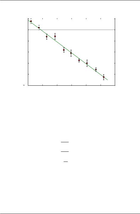
velocity (m/s)
5 |
|
|
Fit to y = ax + b |
|
|
a = 4.4 ± 0.7 m/s |
|
|
|
|
|
|
|
||
0 |
|
|
b = -9.8 ± 0.4 m/s2 |
|
|
χ2 = 0.839 |
|
|
|
|
 5
5
 10
10
 15
15
 20
20
25 |
0.5 |
1.0 |
1.5 |
2.0 |
2.5 |
3.0 |
0.0 |
time (s)
Figure 7.3: Fit using 2 least squares fitting routine with data weighted by error bars.
7.4 Exercises
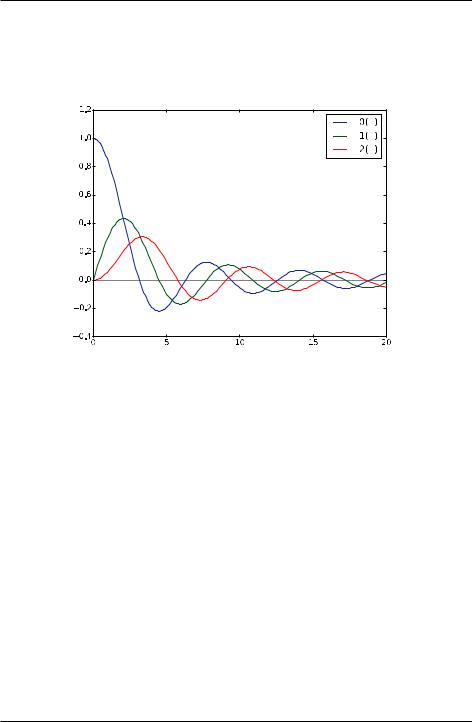
1.Write a function that can return each of the first three spherical Bessel functions jn(x):
j0(x) =
j1(x) =
j2(x) =
sin x
x sin x
x2
3
x2
|
cos x |
|
(7.17) |
||
x |
|
|
|||
1 |
x |
x2 |
|||
|
|
sin x |
|
3 cos x |
|
Your function should take as arguments a NumPy array x and the order n, and should return an array of the designated order n spherical Bessel function. Take care to make sure that your functions behave properly at x = 0.
Demonstrate the use of your function by writing a Python routine that plots the three Bessel functions for 0 x 20. Your plot should look like the one below. Something to think about: You might note that j1(x) can be written in terms of j0(x), and that j2(x) can be written in terms of j1(x) and j0(x). Can you take
136 |
Chapter 7. Functions |
Introduction to Python for Science, Release 0.9.23
advantage of this to write a more efficient function for the calculations of j1(x) and j2(x)?
j |
x |
j |
x |
j |
x |
x |
|
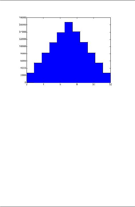
2.(a) Write a function that simulates the rolling of n dice. Use the NumPy function random.random_integers(6), which generates a random integer between 1 and 6 with equal probability (like rolling fair dice). The input of your function should be the number of dice thrown each roll and the output should be the sum of the n dice.
(b)“Roll” 2 dice 10,000 times keeping track of all the sums of each set of rolls in a list. Then use your program to generate a histogram summarizing the rolls of two dice 10,000 times. The result should look like the histogram plotted below. Use the MatPlotLib function hist (see http://matplotlib.org/api/pyplot_summary.html) and set the number of bins in the histogram equal to the number of different possible outcomes of a roll of your dice. For example, the sum of two dice can be anything between 2 and 12, which corresponds to 11 possible outcomes. You should get a histogram that looks like the one below.
(c)“Repeat part (b) using 3 dice and plot the resulting histogram.
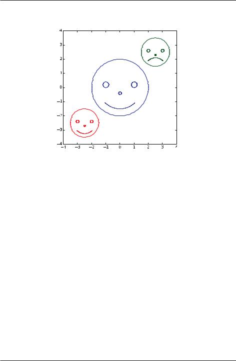
3.Write a function to draw a circular smiley face with eyes, a nose, and a mouth. One argument should set the overall size of the face (the circle radius). Optional arguments should allow the user to specify the (x; y) position of the face, whether
7.4. Exercises |
137 |
Introduction to Python for Science, Release 0.9.23
sum of  dice
dice
the face is smiling or frowning, and the color of the lines. The default should be a smiling blue face centered at (0; 0). Once you write your function, write a program that calls it several times to produce a plot like the one below (creative improvisation is encouraged!). In producing your plot, you may find the call plt.axes().set_aspect(1) useful so that circles appear as circles and not ovals. You should only use MatPlotLib functions introduced in this text. To create a circle you can create an array of angles that goes from 0 to 2 and then produce the x and y arrays for your circle by taking the cosine and sine, respectively, of the array. Hint: You can use the same (x; y) arrays to make the smile and frown as you used to make the circle by plotting appropriate slices of those arrays. You do not need to create new arrays.
4.In the section Example: linear least squares fitting, we showed that the best fit of a line y = a + bx to a set of data f(xi; yi)g is obtained for the values of a and b given by Eq. (7.10). Those formulas were obtained by finding the values of a and b that minimized the sum in Eq. (7.5). This approach and these formulas are valid when the uncertainties in the data are the same for all data points. The Python function
LineFit(x, y) in the section Example: linear least squares fitting implements Eq. (7.10).
(a)Write a new fitting function LineFitWt(x, y) that implements the formulas given in Eq. (7.14) that minimize the 2 function give by Eq. (7.12). This more general approach is valid when the individual data points have dif-
138 |
Chapter 7. Functions |
Introduction to Python for Science, Release 0.9.23
ferent weightings or when they all have the same weighting. You should also write a function to calculate the reduced chi-squared 2r defined by Eq. (7.12).
(b)Write a Python program that reads in the data below, plots it, and fits it using the two fitting functions LineFit(x, y) and LineFitWt(x, y). Your program should plot the data with error bars and with both fits with and without weighting, that is from LineFit(x, y) and LineFitWt(x, y, dy). It should also report the results for both fits on the plot, similar to the output of the supplied program above, as well as the values of 2r, the reduce chi-squared value, for both fits. Explain why weighting the data gives a steeper or less steep slope than the fit without weighting.
Velocity vs time data |
|
|
for a falling mass |
|
|
time (s) |
velocity (m/s) |
uncertainty (m/s) |
2.23 |
139 |
16 |
4.78 |
123 |
16 |
7.21 |
115 |
4 |
9.37 |
96 |
9 |
11.64 |
62 |
17 |
14.23 |
54 |
17 |
16.55 |
10 |
12 |
18.70 |
-3 |
15 |
21.05 |
-13 |
18 |
7.4. Exercises |
139 |

Introduction to Python for Science, Release 0.9.23
23.21 |
-55 |
10 |
5.Modify the function LineFitWt(x, y) you wrote in Exercise 4 above so that in addition to returning the fitting parameters a and b, it also returns the uncertainties in the fitting parameters a and b using the formulas given by Eq. (7.16). Use your new fitting function to find the uncertainties in the fitted slope and y-intercept for the data provided with Exercise 4.
140 |
Chapter 7. Functions |