Introduction to Python for Science, Release 0.9.23

5.5 Exercises

1.Plot the function y = 3x2 for 1 x 3 as a continuous line. Include enough points so that the curve you plot appears smooth. Label the axes x and y.

2.Plot the following function for 15 x 15:

y = cos x 1 + 15 x2

Include enough points so that the curve you plot appears smooth. Label the axes x and y.

3. Plot the functions sin x and cos x vs x on the same plot with x going from to. Make sure the limits of x-axis do not extend beyond the limits of the data. Plot sin x in the color green and cos x in the color black and include a legend to label the two curves. Place the legend within the plot, but such that it does not cover either of the sine or cosine traces.

4.Create a data file with the data shown below.

(a)Read the data into Python program and plot t vs y using circles for data points with error bars. Use the data in the dy column as the error estimates for the y data. Label the horizontal and vertical axes “time (s)” and “position (cm)”.

(b)On the same graph, plot the function below as a smooth line. Make the line pass behind the data points.

Data for Exercise 4

Date: 16-Aug-2013

Data taken by Lauren and John

1.02.94 0.7

4.58.29 1.2

8.09.36 1.2

11.511.60 1.4

15.09.32 1.3

18.57.75 1.1

22.08.06 1.2

25.5 5.60 1.0

Introduction to Python for Science, Release 0.9.23

29.04.50 0.8

32.54.01 0.8

36.02.62 0.7

39.51.70 0.6

43.0 2.03 0.6

5.Use MatPlotLib’s function hist along with NumPy’s function’s random.rand and random.randn to create the histogram graphs shown in Fig. Histograms of random numbers.

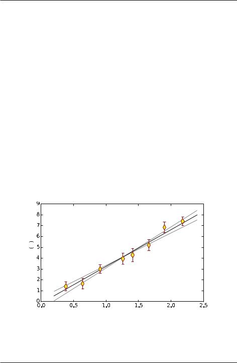
6.Plot force vs distance with error bars using the following data:

d=np.array([0.38, 0.64, 0.91, 1.26, 1.41, 1.66, 1.90, 2.18]) f=np.array([1.4, 1.65, 3.0, 3.95, 4.3, 5.20, 6.85, 7.4]) df=np.array([ 0.4, 0.5, 0.4, 0.5, 0.6, 0.5, 0.5, 0.4])

Your plot should also include a visual straight “best fit” to the data as well as visual “fits” that give the smallest and largest slopes consistent with the data. Note, you only need two points to define a straight line so the straight lines you draw on the plot should be arrays of length 2 and no longer. All of your fitted lines should lie behind the data. Try to make your plot look like the one below. In addition, add a legend to your plot the gives the slope with its uncertainty obtained from your visual fits to the data.

distance cm

The web page http://matplotlib.org/api/pyplot_summary.html gives a summary of the main plotting commands available in MatPlotLib. The two important ones here

Introduction to Python for Science, Release 0.9.23

are plot and errorbar, which make regular plots and plots with error bars, respectively. You will find the following keyword arguments useful: yerr, ls, marker, mfc, mec, ms, and ecolor, which you can find described by clicking on the errorbar function link on the web page cited above.

7.The data file below shows data obtained for the displacement (position) vs time of a falling object, together with the estimated uncertainty in the displacement.

Measurements of fall velocity vs time

Taken by A.P. Crawford and S.M. Torres

(a)Use these data to calculate the velocity and acceleration (in a Python program

.py file), together with their uncertainties propagated from the displacement vs time uncertainties. Be sure to calculate time arrays corresponding the midpoint in time between the two displacements or velocities for the velocity and acceleration arrays, respectively.

(b)In a single window frame, make three vertically stacked plots of the displacement, velocity, and acceleration vs time. Show the error bars on the different plots. Make sure that the time axes of all three plots cover the same range of times. Why do the relative sizes of the error bars grow progressively greater as one progresses from displacement to velocity to acceleration?