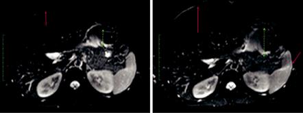
Fig. 1.4  SE-EPI images acquired at 3 T (same image matrix and TR, TE, with b = 0 s/mm2) with anterior to posterior phase encoding direction, EPI echo train length of 41 (left) and 95 (right, with more blurring and larger distortions). The red arrows indicate the water-fat shift (distance between the skin and the liver, suboptimal fat suppression), and the green dotted arrow suggests the amplitude of the EPI spatial distortion. High parallel imaging acceleration factors enable lower echo train lengths that result in images with less artefacts

strength and image SNR, an acceleration factor between 2 and 4 is normally used. Recent progress has been provided by the multi-slice simultaneous excitation technique, which allows diffusion-weighted imaging of the liver accelerated by a factor 2 in addition to parallel imaging [9, 10]. However, its clinical utility hasn’t been demonstrated on the gastrointestinal tract, yet.

1.2.3\ Diffusion Modelling in GI Cancer

Malignant neoplasms often present with a strong perfusion component. The capillary random movement through the diffusion gradients constitutes an intravoxel incoherent motion, IVIM, dephasing the Stejskal-Tanner signal. An adequate model should thus take into account both water diffusion and the pseudo-diffusion from blood capillary flow. One approach is provided by the bi-exponential model [11–16]:

where f is the micro-perfusion fraction, D* is the pseudo-diffusion coefficient linked to micro-perfusion and D is the water true diffusion coefficient in the tissue. The major disadvantage that prohibits routine clinical applications of IVIM is that the bi-exponential model is very prone to signal fitting errors. However, fortunately, in general D* D, and there exists a value b* that

meaning that for b > b*, the attenuation comes from pure diffusion D only. Thus, instead of trying at once to fit the bi-exponential model with three parameters f, D* and D, an approximate strategy called “partial fitting” comprises D calculation by fitting a mono-exponential model to the signal of two or more images with b values larger than b*, typically b* = 150 s/mm2:

1.2.4\ Diffusion Biomarkers Quantification

The ADC value, most often derived from a mono-exponential model, depends on the signal fitting and the available SNR. Artefacts might also significantly influence the fit quality. The slope calculated by the linear regression, giving the ADC, will inevitably be influenced by the signal value measured for each point, especially the points corresponding to the highest b values because these have the most attenuated signal and lowest SNR, therefore are more prone to noise. The fit can be performed pixel by pixel to generate an ADC map but can also be based on ROI signal measurement and of course the definition of the ROI (size, position, homogeneous region or not) plays a crucial role [21]. Note that the mean ADC value in the ROI drawn on the ADC map is not identical to the ADC value computed from the mean signal of the same ROI drawn in all separate b value images because the Eq. (1.4) is non-linear. Globally we can expect a better fit quality if an increasing number of b values are used, at the cost of a longer acquisition duration. At fixed b value and diffusion direction, the acquisition might be repeated, providing an average from a higher number of samples. The number of b values or b directions might also be increased at acquisition; the choice of the b values involved in the fit will finally influence the ADC quantification (Fig. 1.6). A recent technique that can be used to further improve contrast between lesions and background tissue by further attenuating the signal of tissues that are bright on high b values is the so-called computed or synthetic b values (Fig. 1.7).

Various quantification strategies regarding the quantification of imaging biomarkers like ADC have been proposed. The traditional method is to draw a region of interest, either with irregular borders identifying the tumour or use multiple small circular regions of interest sampling many different areas of the tumour. The latter is recruited to overcome potential averaging effects when including the whole tumour in the region of interest from where a mean value of the corresponding biomarker will be calculated. Tumours are typically heterogeneous comprising necrosis, fibrosis, haemorrhage, active proliferative areas, etc. When including all these areas in a single region of interest, important information is destroyed. A more comprehensive way to tackle with tumoural heterogeneity is to perform whole tumour segmentation in three dimensions and calculate the frequency of the biomarker values from all pixels belonging to the tumour. Such a representation is called histogram, and apart from the possibility to visualize tumoural heterogeneity, it is possible to quantify various histogram metrics including min, max, mean, median, variance, standard deviation, percentiles, skewness, kurtosis and others (Fig. 1.8). By quantifying histogram metrics before and after treatment, someone can assess in a comprehensive way how the effect of treatment to the specific biomarker is utilized.

In the clinical setting, a compromise must be found considering the number of slices, the spatial resolution, the use of trigger methods or a breath-hold approach. Of course, a central question is whether the examination aims at lesion detection (ADC map with enough contrast between the lesion and the surrounding tissue) or aims at a precise quantification with low variability, required in the case of a longitudinal study meant to detect a change due to the natural evolution of the disease or being the signature of a response to a treatment.