17.3.2 Radiation from small antennas

Small antennas are needed for mobile communications operating at frequencies from HF to the low microwave region. Most of these are derivatives of the simple dipole, Figure 17.6, which is an electric current element which radiates from the currents flowing along a small metal rod. The radiation pattern is always very broad with energy radiating in all directions. An important design parameter is the impedance of the dipole which can vary considerably depending on the exact size and shape of the rod. This means that the impedance matching between the antenna and the transmitting or receiv­ing circuit becomes a major design constraint. Table 17.2 Radiation characteristics of circular apertures.

The radiation fields from a dipole are obtained by integrating the radiation from an infinitesimally small current element over the length of the dipole. This depends on knowing the current distribu­tion which is a function not only of the length but also of the shape and thickness of the rod. Many studies have been addressed towards obtaining accurate results (King, 1956; King, 1968). For most cases this has to be done by numerical integration. A simple case is a short dipole with a length when the current distribution may be assumed to be triangular. This results in radiated fields of the form given in Equation 17.9.

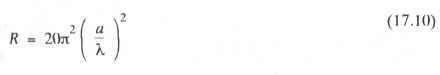
The electric field is plotted in polar form in Figure 17.6. The radiation resistance is calculated by evaluating the radiated power and using P = I²R to give Equation 17.10.

A dipole of length has a radiation resistance of 2.0ohms.

This is low by comparison with standard transmission lines and indicates the problem of matching to the transmission line.

The half wave dipole is widely used. Assuming a sinusoidal current distribution the far fields are given by Equation 17.11.

This gives a slightly narrower pattern than that of the short dipole and has a half beamwidlh of 78 degrees. The radiation resistance must be evaluated numerically. For an infinitely thin dipole it has a value of 73 +j 42.5 ohms. For finite thickness the imaginary part can become zero in which case the dipole is easily matched to a coaxial cable of impedance 75ohms. The half wave dipole has a gain of2.15dB.

A monopole is a dipole divided in half at its centre feed point and fed against a ground plane, Figure 17.6. The ground plane acts as a mirror and consequently the image of the monopole appears below the ground. Since the fields extend over a hemisphere the power radiated and the radiation resistance is half that of the equivalent dipole with the same current. The gain of a monopole is twice that of a dipole. The radiation pattern above the ground plane is the same as that of the dipole.

17.3.3 Radiation from arrays

Array antennas consist of a number of discrete elements which are usually small in size. Typical elements are horns, dipoles, and microchip patches. The discrete sources radiate individually but the pattern of the array is largely determined by the relative amplitude and phase of the excitation currents on each element and the geome­tric spacing apart of the elements. The total radiation pattern is the multiplication of the pattern of an individual element and the pattern of the array assuming point sources, called the array factor. Array theory is largely concerned with synthesising an array factor to form a specified pattern. In communications most arrays are planar arrays with the elements being spaced over a plane, but the principles can be understood by considering an array of two elements with equal amplitudes, Figure 17.7(a). This has an array factor given by Equa­tion 17.12, where ψ is given by Equation 17.13.

The pattern for small spacings will he almost omnidirectional and as the spacing is increased the pattern develops a maxima perpen­dicular to the axis of the array. At a spacing of half a wavelength, a null appears along the array axis. Figure I7.7(b). This is called a broadside array. If a phase difference of 180 degrees exists between the two elements then the pattern shown in Figure I7.7(c) results. Now the main beam is along the direction of the array and the array is called the end-fire array. This illustrates one of the prime advant­ages of the array, namely by changing the electrical phase it is possible to make the peak beam direction occur in any angular direction. Increasing the spacing above half a wavelength results in the appearance of additional radiation lobes which are generally undesirable. Consequently the ideal arrays spacing is half wave­length, though if waveguides or horns are used this is not usually possible because the basic element is greater than half a wavelength in size. Changing the relative amplitudes, phases and spacings can produce a wide variety of patterns so that it is possible to synthesise almost any specified radiation pattern. The array factor for an N element linear array of equal amplitude is given by Equation 17.14.

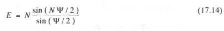
This is similar to the pattern of a line source aperture, Equation 17.5, and it is possible to synthesise an aperture with a planar array. There is a significant benefit to this approach. The aperture fields are determined by the waveguide horn fields which are constrained by boundary conditions and are usually monotonic functions. This constraint does not exist with the array so that a much larger range of radiation patterns can be produced. Optimum patterns with most of the energy radiated into the main beam and very low sidelobes can be designed.