

Embedded Systems Design - An Introduction to Processes Tools and Techniques (A. Berger, 2002)
.pdfinto empty space, the system crashes. Crashes in embedded systems that are not deterministic (such as a bug in the code) are extremely difficult to find. In fact, it might be years before this particular defect causes a failure.
In The Art of Embedded Systems, Jack Ganssle[1] suggests that during system development and debug, you fill the stack space with a known pattern, such as 0x5555 or 0xAA. Run the program for a while and see how much of this pattern has been overwritten by stack operations. Then, add a safety factor (2X, perhaps) to allow for unintended stack growth. The fact that available RAM memory could be an issue might have an impact on the type of programming methods you use or an influence on the hardware design.
System Startup
Understanding the layout of memory makes it easier to understand the startup sequence. This section assumes the device’s program has been loaded into the proper memory space — perhaps by “burning” it into erasable, programmable, read-only memory (EPROM) and then plugging that EPROM into the system board. Other mechanisms for getting the code into the target are discussed later.
The startup sequence has two phases: a hardware phase and a software phase. When the RESET line is activated, the processor executes the hardware phase. The primary responsibility of this part is to force the CPU to begin executing the program or some code that will transfer control to the program. The first few
instructions in the program define the software phase of the startup. The software |
|||
|
|
Y |
|
phase is responsible for initializing core elements of the hardware and key |
|||
structures in memory. |
L |
||
F |
|||
|
|||
For example, when a 68K microprocessor first comes out of RESET, it does two |
|||
|
M |
|
|
things before executing any instructions. First, it fetches the address stored in the |
|||
4 bytes beginning at location 000000Aand copies this address into the stack pointer |
|||
(SP) register, thus establishing the bottom of the stack. It is common for this value |
|||
|
E |
|
|
to be initialized to the top of RAM (e.g., 0XFFFFFFFE) because the stack grows |
|||
down toward memory locationT000000. Next, it fetches the address stored in the |
|||
four bytes at memory location 000004–000007 and places this 32-bit value in its program counter register. This register always points to the memory location of the next instruction to be executed. Finally, the processor fetches the instruction located at the memory address contained in the program counter register and begins executing the program.
At this point, the CPU has begun the software startup phase. The CPU is under control of the software but is probably not ready to execute the application proper. Instead, it executes a block of code that initializes various hardware resources and the data structures necessary to create a complete run-time environment. This “startup code” is described in more detail later.
Interrupt Response Cycle
Conceptually, interrupts are relatively simple: When an interrupt signal is received, the CPU “sets aside” what it is doing, executes the instructions necessary to take care of the interrupt, and then resumes its previous task. The critical element is that the CPU hardware must take care of transferring control from one task to the other and back. The developer can’t code this transfer into the normal instruction stream because there is no way to predict when the interrupt signal will be received. Although this transfer mechanism is almost the same on all architectures,
Team-Fly®
small significant differences exist among how different CPUs handle the details. The key issues to understand are:
How does the CPU know where to find the interrupt handling code?
What does it take to save and restore the “context” of the main thread?
When should interrupts be enabled?
As mentioned previously, a 68K CPU expects the first 1024 bytes of memory to hold a table of exception vectors, that is, addresses. The first of these is the address to load into SP during system RESET. The second is the address to load into the program counter register during RESET. The rest of the 254 long addresses in the exception vector table contain pointers to the starting address of exception routines, one for each kind of exception that the 68K is capable of generating or recognizing. Some of these are connected to the interrupts discussed in this section, while others are associated with other anomalies (such as an attempt to divide by zero) which may occur during normal code execution.
When a device[1] asserts an interrupt signal to the CPU (if the CPU is able to accept the interrupt), the 68K will:
Push the address of the next instruction (the return address) onto the stack.
Load the ISR address (vector) from the exception table into the program counter.
Disable interrupts.
Resume executing normal fetch–execute cycles. At this point, however, it is fetching instructions that belong to the ISR.
This response is deliberately similar to what happens when the processor executes a call or jump to subroutine (JSR) instruction. (In fact, on some CPUs, it is identical.) You can think of the interrupt response as a hardwareinvoked function call in which the address of the target function is pulled from the exception vector. To resume the main program, the programmer must terminate the ISR with a return from subroutine (RTS) instruction, just as one would return from a function. (Some machines require you to use a special return from interrupt [RTE, return from exception on the 68k] instruction.)
ISRs are discussed in more detail in the next chapter. For now, it’s enough to think of them as hardware-invoked functions. Function calls, hardware or software, are more complex to implement than indicated here.
[1]In the case of a microcontroller, an external device could be internal to the chip but exter nal to the CPU core.
Function Calls and Stack Frames
When you write a C function and assemble it, the compiler converts it to an assembly language subroutine. The name of the assembly language subroutine is just the function name preceded by an underscore character. For example, main()
becomes _main. Just as the C function main() is terminated by a return statement, the assembly language version is terminated by the assembly language equivalent: RTS.
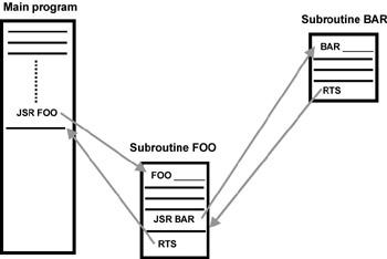
Figure 4.2 shows two subroutines, FOO and BAR, one nested inside of the other. The main program calls subroutine FOO which then calls subroutine BAR. The compiler translates the call to BAR using the same mechanism as for the call to FOO. The automatic placing and retrieval of addresses from the stack is possible because the stack is set up as a last- in/first-out data structure. You PUSH return addresses onto the stack and then POP them from the stack to return from the function call.
Figure 4.2: Subroutines.
Schematic representation of the structure of an assembly-language subroutine.
The assembly-language subroutine is “called” with a JSR assembly language instruction. The argument of the instruction is the memory address of the start of the subroutine. When the processor executes the JSR instruction, it automatically places the address of the next instruction — that is, the address of the instruction immediately following the JSR instruction — on the processor stack. (Compare this to the interrupt response cycle discussed previously.) First the CPU decrements the SP to point to the next available stack location. (Remember that on the 68K the SP register grows downward in memory.) Then the processor writes the return address to the stack (to the address now in SP).
Hint A very instructive experiment that you should be able to perform with any embedded C compiler is to write a simple C program and compile it with a “compile only” option. This should cause the compiler to generate an assembly language listing file. If you open this assembly file in an editor, you’ll see the various C statements along with the assembly language statements that are generated. The C statements appear as comments in the assembly language source file.
Some argue that generating assembly is obsolete. Many modern compilers skip the assembly language step entirely and go from compiler directly to object code. If you want to see the assembly language output of the compiler, you set a compiler option switch that causes a disassembly of the object file to create an assembly language source file. Thus, assembly language is not part of the process.
The next instruction begins execution at the starting address of the subroutine (function). Program execution continues from this new location until the RTS instruction is encountered. The RTS instruction causes the address stored on the stack to be automatically retrieved from the stack and placed in the program counter register, where program execution now resumes from the instruction following the JSR instruction.
The stack is also used to store all of a function’s local variables and arguments. Although return addresses are managed implicitly by the hardware each time a JSR or RTS is executed, the compiler must generate explicit assembly language to manage local variable storage. Here, different compilers can choose different options. Generally, the compiler must generate code to
Push all arguments onto the stack
Call the function
Allocate storage (on the stack) for all local variables
Perform the work of the function
Deallocate the local variable storage
Return from the function
Deallocate the space used by the arguments
The collection of all space allocated for a single function call (arguments, return addresses, and local variables) is called a stack frame. To simplify access to the arguments and local variables, at each function entry, the compiler generates code that loads a pointer to the current function’s stack frame into a processor register
— typically called Frame Pointer (FP). Thus, within the assembly language subroutine, a stack frame is nothing more than a local block of RAM that must be addressed via one of the CPU’s internal address registers (FP).
A complete description of a stack frame includes more than locals, parameters, and return addresses. To simplify call nesting, the old FP is pushed onto the stack each time a function is called. Also, the "working values" in certain registers might need to be saved (also in the stack) to keep them from being overwritten by the called function. Thus, every time the compiler encounters a function call, it must potentially generate quite a bit of code (called "prolog" and "epilogue") to support creating and destroying a local stack frame. Many CPUs include special instructions designed to improve the efficiency of this process. The 68K processor, for example, includes two instructions, link and unlink (LNK and UNLNK) that were created especially to support the creation of C stack frames.
Run-Time Environment
Just as the execution environment comprises all the hardware facilities that support program execution, the run-time environment consists of all the software structures (not explicitly created by the programmer) that support program execution. Although I’ve already discussed the stack and stack frames as part of the execution environment, the structure linking stack frames also can be considered a significant part of the run-time environment. For C programmers, two other major components comprise the runtime environment: the startup code and the run-time library.
Startup Code
Startup code is the software that bridges the connection between the hardware startup phase and the program’s main(). This bridging software should be executed at each RESET and, at a minimum, should transfer control to main(). Thus, a trivial implementation might consist of an assembly language file containing the single instruction:JMP _main
To make this code execute at startup, you also need to find a way to store the address of this JMP into memory locations 000004–000007 (the exception vector for the first instruction to be executed by the processor.) I’ll explain how to accomplish that later in the section on linkers.
Typically, however, you wouldn’t want the program to jump immediately to main(). A real system, when it first starts up, will probably do some system integrity checks, such as run a ROM checksum test, run a RAM test, relocate code stored in ROM to RAM for faster access, initialize hardware registers, and set up the rest of the C environment before jumping to _main. Whereas in a desktop environment, the startup code never needs to be changed, in an embedded environment, the startup code needs to be customized for every different board. To make it easy to modify the startup behavior, most embedded market C compilers automatically generate code to include a separate assembly language file that contains the startup code. Typically, this file is named crt0 or crt1 (where crt is short for C Run Time). This convention allows the embedded developer to modify the startup code separately (usually as part of building the board support package).
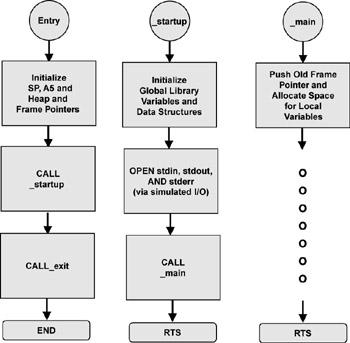
Figure 4.3 shows the flowchart for the crt0 function for the HewlettPackard B3640 68K Family C Cross Compiler.
Figure 4.3: crt0 function
The crt0 program setup flowchart.[2]
Why JMP_main Was Used
You might be wondering why I used the instruction JMP_main and not the instruction JSR _main. First of all, JSR_main implies that after it’s done running main(), it returns to the calling routine. Where is the calling routine? In this case, main() is the starting and ending point. Once it is running, it runs forever. Thus, function main() might look like this pseudocode representation:
main()
{
Initialize variables and get ready to run;
While(1)
{
Rest of the program here;
}
return 0;
}
After you enter the while loop, you stay there forever. Thus, a JMP _main is as good as a JSR _main.
However, not all programs run in isolation. Just like a desktop application runs under Windows or UNIX, an embedded application can run under an embedded operating system, for example, a RTOS such as VxWorks. With an RTOS in control of your environment, a C program or task might terminate and control would have to be returned to the operating system. In this case, it is appropriate to enter the function main() with a JSR _main.
This is just one example of how the startup code might need to be adjusted for a given project.
The Run-Time Library
In the most restrictive definition, the run-time library is a set of otherwise invisible support functions that simplify code generation. For example, on a machine that doesn’t have hardware support for floating-point operations, the compiler generates a call to an arithmetic routine in the run-time library for each floatingpoint operation. On machines with awkward register structures, sometimes the compiler generates a call to a context-saving routine instead of trying to generate code that explicitly saves each register.
For this discussion, consider the routines in the C standard library to be part of the run-time library. (In fact, the compiler run-time support might be packaged in the same library module with the core standard library functions.)
The run-time library becomes an issue in embedded systems development primarily because of resource constraints. By eliminating unneeded or seldom used functions from the run-time library, you can reduce the load size of the program.
You can get similar reductions by replacing complex implementations with simple ones.
These kinds of optimizations usually affect three facilities that application programmers tend to take for granted: floating-point support, formatted output (printf()), and dynamic allocation support (malloc() and C++’s new). Typically, if one of these features has been omitted, the embedded development environment supplies some simpler, less code-intensive alternative. For example, if no floatingpoint support exists, the compiler vendor might supply a fixed-point library that you can call explicitly. Instead of full printf() support, the vendor might supply functions to format specific types (for example, printIntAsHex(), printStr(), and so on).
Dynamic allocation, however, is a little different. How, or even if, you implement dynamic allocation depends on many factors other than available code space and hardware support. If the system is running under an RTOS, the allocation system will likely be controlled by the RTOS. The developer will usually need to customize the lower level functions (such as the getmem() function discussed in the following) to adapt the RTOS to the particular memory configuration of the target system. If the system is safety critical, the allocation system must be very robust. Because allocation routines can impose significant execution overhead, processor-bound systems might need to employ special, fast algorithms.
Many systems won’t have enough RAM to support dynamic allocation. Even those that do might be better off without it. Dynamic memory allocation is not commonly used in embedded systems because of the dangers inherent in unexpectedly running out of memory due to using it up or to fragmentation issues. Moreover, algorithms based on dynamically allocated structures tend to be more difficult to test and debug than algorithms based on static structures.
Most RTOSs supply memory-management functions. However, unless your target system is a standard platform, you should plan on rewriting some of the malloc() function to customize it for your environment. At a minimum, the cross-compiler that might be used with an embedded system needs to know about the system’s memory model.
For example, the HP compiler discussed earlier isolates the system-specific information in an assembly language function called _getmem(). In the HP implementation, _getmem() returns the address of a block of memory and the size of that block. If the size of the returned block cannot meet the requested size, the biggest available block is returned. The user is responsible for modifying this getmem() according to the requirements of the particular target system. Although HP supplies a generic implementation for getmem(), you are expected to rewrite it to fit the needs and capabilities of your system.
Note You can find more information about dynamic allocation in embedded system projects in these articles:
Dailey, Aaron. “Effective C++ Memory Allocation.” Embedded Systems Programming, January 1999, 44.
Hogaboom, Richard. “Flexible Dynamic Array Allocation.” Embedded Systems Programming, December 2000, 152.
Ivanovic, Vladimir G. “Java and C++: A Language Comparison.” Real Time Computing, March 1998, 75.
Lafreniere, David. “An Efficient Dynamic Storage Allocator.” Embedded Systems Programming, September 1998, 72.
Murphy, Niall. “Safe Memory Utilization.” Embedded Systems Programming, April 2000, 110.
Shaw, Kent. “Run-Time Error Checking,” Embedded Developers Journal, May 2000, 8.
Stewart, David B. “More Pitfalls for Real-Time Software Developers.”
Embedded Systems Programming, November 1999, 74.
Object Placement
It should be clear by now that an embedded systems programmer needs to be able to control the physical position of code and data in memory. To create a table of exception vectors, for example, you must be able to create an array of ISR addresses and force it to reside at location zero. Similarly, embedded systems programmers must be able to force program instructions to reside at an address corresponding to EPROM and to force global data to reside at addresses corresponding to RAM. Startup code and ISRs pose similar challenges.
The linker is the primary tool for controlling code placement. Generally, the assembler creates relocatable modules that the linker “fixes” at specific physical addresses. The following sections explain relocatable modules and how the embedded systems programmer can exercise control over the physical placement of objects.
Relocatable Objects
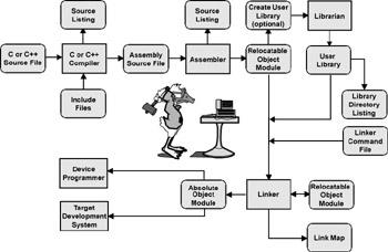
Figure 4.4 represents the classical development model. The C or C++ source file and include files are compiled into an assembly language source file and then the assembler creates a relocatable object file.
Figure 4.4: Embedded software development process.
A road map for the creation and design of embedded software.
As the assembler translates the source modules, it maintains an internal counter — the location counter — to keep track of the instruction boundaries, relative to the starting address of the block.
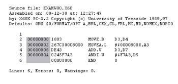
Figure 4.5 is a snippet of 68K assembly language code. The byte count corresponding to the current value of the location counter is highlighted in Figure 4.5. The counter shows the address of the instructions in this block of code, although it could just as easily show the relative byte counts (offsets) for data blocks. In the simplest development environments, the developer uses special assembly language pseudo-instructions to place objects at particular locations (such as ORG 200H to start a module at address 512.) When working in a higherlevel language, you need some other mechanism for controlling placement.
Figure 4.5: Assembly lafnguage snippet.
In this snippet of 68K assembly-language code, the location counter is highlighted.
The solution is to have the assembler generate relocatable modules. Each relocatable module is translated as if it will reside at location zero. When the assembler prepares the module, it also prepares a symbol table showing which values in the module will need to change if the module is moved to some location other than zero. Before loading these modules for execution, the linker relocates them, that is, it adjusts all the position-sensitive values to be appropriate for where the module actually will reside. Modern instruction sets often include instructions specifically designed to simplify the linker’s job (for example, “jumprelative” instructions, which do not need adjusting). Often, the compilers and linkers for such machines can be instructed to generate position-independent code (PIC), which requires no adjustments, regardless of where the code will ultimately reside in memory.
The relocatable modules (or files) typically reference functions in other modules, so, at first glance, you have a Pandora’s box of interconnected function calls and memory references. In addition to adjusting internal references for actual location, the linker is also responsible for resolving these inter-module references and creating a block of code that can be loaded into a specific location in the system.
Advantages of Relocatable Modules
Relocatable modules are important for many reasons. For the embedded systems programmer, relocatable modules simplify the physical placement of code generated from a high-level language and allow individual modules to be independently updated and recompiled.
In general-purpose systems, relocatable modules have the added benefits of simplifying memory management (by allowing individual programs to be loaded into any available section of memory without recompilation) and facilitating the use of shared, precompiled libraries.
Using the Linker
The inputs to the linker are the relocatable object modules and the linker command file. The linker command file gives the software engineer complete control of how the code modules are linked together to create the final image. The linker command file is a key element in this process and is an important differentiator between writing code for an embedded system and a desktop PC. The linker command file is a user-created text file that tells the linker how the
relocatable object modules are to be linked together. Linkers use program sections. A program section is a block of code or data that is logically distinct from other sections and can be described by its own location counter.
Sections have various attributes that tell the linker how they are to be used. For example, a section might be:
Program code
Program data
Mixed code and data
ROMable data
Listing 4.1 shows a typical Motorola 68K family linker command file. The meanings of the linker commands are explained in Table 4.1.
Table 4.1: Linker commands.
CHIP
specifies the target microprocessor. It also determines how sections are aligned on memory address boundaries and, depending upon the microprocessor specified, how much memory space is available. Finally, it determines the behavior of certain processor-specific addressing modes.
LISTMAP
generates a symbol table listing both local and external definition symbols. It also causes these symbols to be placed in the output object module so that a debugger can associate symbols with memory addresses later on. The symbol table displays the symbols along with their final absolute address locations. You can look at the link map output and determine whether all the modules were linked properly and will reside in memory where you think they should be. If the linker was successful, all addresses are adjusted to their proper final values and all links between modules are resolved.
COMMON; named COMSEC
is placed at hexadecimal starting address 1000 ($ means hexadecimal). The linker places all COMMON sections from different modules with the same name in the same place in memory. COMMON sections are generally used for program variables that will reside in RAM, such as global variables.
ORDER
specifies the order that the sections are linked together into the executable image.
PUBLIC
specifies an absolute address, hexadecimal 2000, for the variable EXTRANEOUS. This is an interesting command, and I’ll return to it in Chapter 5, when I discuss