Embedded Systems Design - An Introduction to Processes Tools and Techniques (A. Berger, 2002)

saving the memory from recording uninteresting tasks. The logic analyzer’s trigger system is usually arranged around the concept of resources and state transitions.

Tip It’s helpful to record only several states before and after accesses to a certain memory location. In other words, every time a global variable is accessed, a limited number of states around it are recorded. This allows you to easily isolate why the global variable was being mysteriously clobbered by another task.

Trigger Resources

The logic analyzer’s trigger system is usually arranged around the concept of resources and state transitions. Think of the resources as logic variables. A resource might be assigned to a condition of the system, such as ADDRESS = 0x5555AAAA. However, just as with C, you can assign a resource so that ADDRESS != 0x5555AAAA. In other words, trigger if the address doesn’t equal this value. You also can assign ranges to resources, so that if the address bus has a value in the range of

0x50000000 <= ADDRESS <= 0x50000010

the logic analyzer triggers. You can also trigger on addresses outside a specific range, as in

the logic analyzer only uses address bits 20 through 31 in the comparison and ignores bits 0 through 19. In a way, this is similar to declaring a range trigger but without defining an explicit range. Most logic analyzers support a fixed number of resources that can be assigned to trigger conditions. To create a range resource, you must combine two resources so that the trigger occurs on the logical ANDing of RESOURCE1 (0x50000000 <= ADDRESS) and RESOURCE2 (ADDRESS <= 0x50000010).

You also can assign trigger resources to the data bus bits and to the status bus bits. Just as you can logically AND to address resources to create an address range trigger condition, you can create logical AND, OR, and NOT combinations of the processor’s buses or individual bits. Thus, one might form a complex trigger condition like this:

IF (ADDRESS=0xAAAAAAAA) AND (DATA=0x0034) AND (STATUS=WRITE) THEN TRIGGER.

Tip Programmers often need to debug with loop problems present. Either the loop occurs an infinite number of times, one time too few, one time too many, or all of the above. If the loop is a polling loop waiting for a hardware event to occur, for example, just triggering on the address condition of entering the loop quickly fills up the logic analyzer memory buffer without capturing the event of interest. The logic analyzer can get around loop problems by providing an internal counter that keeps track of the number of times an address or data value occurs. The trace then triggers after the counter reaches the preset value. Thus, if you are

Team-Fly®

interested in the exit value of a loop that should have occurred 500 times, you might set the counter to trigger on the address value after 495 times.

How Triggers Work

To understand a trigger, recall that the logic analyzer is a passive device. It records the signals that appear on the microprocessor busses while the processor runs normally. Because the processor might be executing 10 million or more instructions each second and the logic analyzer has finite memory, you need a mechanism to tell the trace memory when to start and stop storing state or timing information. By turning the recording on at the appropriate time, you can record (capture) the actions of the processor around the point of interest. So, just as you use a debugger to set breakpoints in your code, you can use the trigger capabilities of a logic analyzer to record the instruction and data flow at some point in the program execution flow.

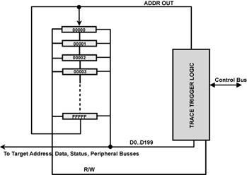
The schematic diagram in Figures 6.15 represents a memory system that is one million states deep and 200 bits wide. It is arranged as a circular buffer so that no special significance to memory location 0x00000 or 0xFFFFF exists; they just are adjacent to each other in the buffer. Each time the processor clock is asserted — usually on a rising edge — 200 bits are recorded in the memory, and the address is automatically incremented to the next location.

This process goes on continuously, whether the logic analyzer is supposed to record any information or not. After it records one million states, the logic analyzer just records over what it previously recorded. The key contribution of the trigger circuitry is to tell the logic analyzer trigger when to stop recording information. This simple concept has some powerful debugging implications. With the logic analyzer set up this way, you can see backward in time, up to 1 million states before the trigger signal occurs.

Figure 6.15: Memory system diagram.

Schematic representation of a logic analyzer trace and trigger system.

State Transitions

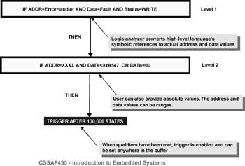
Recall that one of the real problems with debugging code is isolating and capturing the event of interest among a complex array of possible pathways. Sometimes specifying address, data, and status values, even with the capability of defining complicated patterns, is just not enough. This is where the state transition trigger capability can be used (see Figure 6.16). With trigger sequencing, the resources have been combined to provide a triggering capability that depends on the path taken through the code.

Figure 6.16: Triggers.

Triggering a logic analyzer after a sequence of trigger states.

Each match that occurs takes you to a new level in the trigger-sequencing system. Eventually, if all the transition conditions are met, the logic analyzer triggers. Setting up such a complex combination of trigger conditions isn’t a task for the faint of heart. It usually takes a lot of trial and error before you get the trigger system working properly. Unfortunately, your ability to get the most out of the logic analyzer’s triggering capability is often greatly diminished by the logic analyzer’s user interface, documentation, or both. It is extremely frustrating when you know exactly what you want to do, but can’t figure out how to make your tool do it.

With a logic analyzer, this often means that you set it up to trigger on some complex, low-occurrence fault — occurring perhaps once a day — and you miss the event because your trigger sequence was set incorrectly. The sad reality is that most engineers hardly ever take advantage of the logic analyzer’s complex triggering capabilities because it is just too difficult to set up the logic analyzer with any confidence that you’ll be successful the first time you try it.

From the Trenches

I visited a customer once to learn more about how our products were being used. Our logic analyzer had extremely powerful triggering capabilities, a rich set of resources, and eight levels of trigger sequencing. Referring back to Figure 6.16, imagine up to eight of those logical conditions with various kinds of looping back to prior states. The logic analyzer did not have a particularly deep memory and could store a maximum of 1,024 states, which was a source of constant complaint by the customers we visited. The memory was just not deep enough. We would counter their argument by saying that the complex triggering capability made a deep memory unnecessary. Just dial in the trigger condition that you need to isolate the

fault, and then you won’t need to search through a deep memory buffer for the event, which you have to do if your trigger condition is too simple.

Most, if not all, the customers wanted a simple trigger to capture the event, and then they were willing to search manually through the trace buffer for the event of interest. Several, in fact, were proud of some utilities they wrote to post-process the trace file from the logic analyzer. Because they could upload it as an ASCII text file, they wrote software to find the trace event that they were interested in.

Customer research shows that 90 percent of users triggered their logic analyzer (or ICE) on simple Boolean combinations of address, data, and status information, with perhaps a count qualifier added for loop unrolling.

This apparent disconnect between what the user needs (simple triggering with a deep trace and post-processing) and what the tool vendor supplies (complex triggering with shallow memory) reflects the logic analyzer’s roots as a hardware designer’s tool. State sequencing is a common algorithm for a hardware designer but less well known for a software developer. Tools such as oscilloscopes and logic analyzers are created by hardware designers for hardware designers. Thus, it’s easy to understand the focus on state sequencing as the triggering architecture. In any case, the logic analyzer is a powerful tool for debugging real-time systems. Although this chapter has concentrated on the processor’s busses, the logic analyzer easily can measure other signals in your digital system along with the processor so you can see what peripheral devices are doing as the processor attempts to deal with them.

Limitations

By now, you might think the logic analyzer is the greatest thing since sliced bread. What’s the down side? The first hurdle is the problem of mechanical connections between the logic analyzer and the target system. If you’ve every tried to measure a voltage in a circuit, you know that to measure one voltage, you need two probes. One probe connects to the source of the voltage and the other connects to the circuit ground to bring your voltmeter and the circuit to the same reference point. If your processor has 200 I/O pins, which is reasonably common today, you need to be able to make 201 connections to the processor to capture all its I/O signals.

The second problem is that meaningful interpretation of a logic analyzer trace assumes you can relate the addresses and data observed on the bus to sequences of instruction executions. Unfortunately, the on-chip cache and other performance enhancements (such as out-of-order instruction dispatch) interfere with this assumption.

Physical Connections

Logic analyzer manufacturers are painfully aware of the difficulty associated with connecting several hundred microscopic I/O pins to their tools and have built interconnecting systems that enable the logic analyzer and a surface-mounted microprocessor to make a reasonable electrical and mechanical connection. These interconnecting devices are often called preprocessors. For relatively simple pingrid array packages, where the I/O pins of the processor are designed to plug into a socket with a two-dimensional array of holes located on 0.1 inch centers, the preprocessor plugs into the socket on the target system, and the target microprocessor plugs into the preprocessor. This arrangement is also referred to as an interposer because the preprocessor sits between the target and the processor.

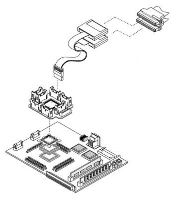
Figure 6.17 shows an example of a preprocessor. The preprocessor can contain some additional circuitry (such as the transition board shown in Figure 6.10) to provide some signal isolation because of the added electrical load created by the preprocessor and the logic analyzer. If you’re unlucky and your embedded processor is more like the ColdFIRE chip shown in Figure 6.17, the preprocessor could be a rather fragile and expensive device. In one design, a threaded bolt is glued to the top of the plastic IC package using a special alignment jig and cyanoacrylic glue. The rest of the connector then attaches to this stud and positions the mini-probes on the I/O pins of the processor. It takes a bit of trial and error to get all the preprocessor connections made, but the preprocessor is reliable after it’s installed. However, this is not something that you want to attach and remove from the chip at regular intervals.

Figure 6.17: Preprocessor connection sequence.

The preprocessor provides over 100 reliable electrical and mechanical connections to the target processor and to the logic analyzer. Drawing courtesy of Agilent Technologies, Inc.

From the Trenches

One company keeps these expensive connectors in a locked cabinet. The group’s manager has the key, and engineers are allowed one free replacement. After that, each subsequent replacement requires more and more in-depth analysis of the engineer’s design and debugging methods.

Logic Analyzers and Caches

Now that you have this expensive preprocessor probe connected to the microprocessor and you’re ready to debug, you might be out of the woods. Suppose your embedded microprocessor has an input pipeline or an on-chip instruction cache (I-cache), data cache (D-cache), or both. It definitely makes triggering a logic analyzer and capturing a trace a much more problematic task.

Remember that the logic analyzer is passively “sniffing” the processor’s I/O pins on every clock cycle. If every state that is visible on the bus corresponds to what the processor is doing with that instruction, the logic analyzer will accurately capture the instruction and data flow sequence of the processor.

However, if the activity on the bus does not have a 1:1 correspondence to the instructions being executed and the data being accessed, the logic analyzer’s usefulness begins to diminish. Most on-chip caches are generally refilled from main memory in bursts. Even if only one byte of data is not available in the cache, the bus control logic of the processor generally fetches anywhere from 4 to 64 bytes of data, called a refill line, from main memory and places the refill line in the cache. The logic analyzer records a burst of memory reads taking place. Where’s the data of interest?

If the caches are small, clever post-processing software can sometimes figure out what the processor is actually doing and display the real flow. You might still have a problem with triggering, but it’s possible to circumvent it. With small caches, branches in the code generally have at least one possible branch destination located outside the cache. Thus, clever software might be able to use basic block information from the compiler and the address of memory fetches to reconstruct what happened at various branch points. If the caches are large enough to normally hold both possible destinations of a branch, a logic analyzer, with only external bus information available to it, has no way to determine what instructions are being executed by the processor. Of course, most processors allow you to set a bit in a register and turn off the caches. However, as with the debug kernel discussed earlier, the performance degradation caused by the intrusion of the logic analyzer might cause your embedded system to fail or to behave differently than it would if the caches were enabled.

Trace Visibility

Most manufactures of embedded systems understand the importance of real-time traces and add on-chip circuitry to help logic analyzers or other tools decode what is actually going on inside of the processor. Over the years, several different approaches have been taken. National Semiconductor Corporation and Intel Corporation created special versions of their embedded processors called “bondouts” because additional signals that were available on the integrated circuit die were bonded out to extra I/O pins on these special packages. Thus, a normal package might have 100 pins, but the bond-out version has 140 pins. These extra pins provided additional information about the program counter and cache behavior. With this information, it becomes feasible to post-process the logic analyzer trace to uncover the processor program flow.

Traceable Cache™

AMD took another approach called Traceable Cache™. Rather than create a bondout version of the chip, certain AMD 29K family processors could be put into a slave mode through the JTAG port. The master processor and slave processor are mounted together on a preprocessor module, and both have their data lines connected to the system data bus. Only the master processor has its address lines connected to the address bus. The two microprocessors then run in lockstep. The unconnected address pins of the slave processor output the current value of the program counter on every instruction cycle. These additional states are captured by the logic analyzer, and, by post-processing the resulting trace, the actual instruction flow can be reconstructed, even though the processor is running out of the cache.

Today, the generally accepted method of providing trace information is to output the program counter value when a non-sequential fetch occurs. A non-sequential fetch occurs whenever the program counter is not incremented to point to the address of the next instruction in memory. A branch, a loop, a jump to subroutine, or an interrupt causes non-sequential fetches to occur. If the debug tools record all the non-sequential fetches, they should be able to reconstruct the instruction flow, but not the data flow, of the processor. Non-sequential fetch information can be output when the bus is idle, so it usually has a minimal impact on the processor’s performance; however, tight loops can often cause problems if the data is coming too fast. Some sort of an on-chip FIFO for the non-sequential fetch data usually helps here, but even that can get overrun if the branch destination is being output every few clock cycles.

Caches and Triggering

As noted earlier, triggering might still be a problem. Traditional triggering methods also fail when caches are present, so the semiconductor manufacturers place triggering resources on-chip, as part of their debug circuitry. Often, these resources are called breakpoint registers because they are also available to debuggers for setting breakpoints in the code. A breakpoint register might be set to cause a special code to be output on several status pins whenever the internal breakpoint conditions are met. The code is then interpreted by the logic analyzer as a trigger signal, and the logic analyzer takes the appropriate action, such as starting to capture a trace. Chapter 7 discusses the IEEE ISTO-5001 embedded debug standard, including the various dynamic debugging modes defined in the standard.

In these examples, you’ve seen that as the processor speed and complexity increases, the type of information that you must record to understand what the processor is doing necessarily changes as well. Today, attempting to capture the external bus states on every clock cycle is generally not possible or necessary. By effectively using the on-chip dynamic debug resources, such as the address information about non-sequential fetched and internal trigger resources, you usually can record enough information from the processor to reconstruct the realtime instruction flow of the processor.

Compiler Optimizations

With optimizations turned on, a good C or C++ compiler can generate code that, at the assembly language level, is almost impossible to relate to the original source code. Even with the C source statements interspersed with the assembly code, critical events might not show up in the trace where you expect them to be. Of course, turning off the optimizations can have the same effect as turning off the caches to gain visibility. The tool becomes intrusive, and performance is compromised, perhaps so much as to cause the embedded system to fail.

Cost Benefit

Even with all the limitations of logic analysis as a debugging tool, the negatives don’t outweigh the positives. Although high-performance logic analyzers can be expensive (over $20,000), excellent units are available below $10,000 that will meet your needs for a long time to come. Magazines, such as Electronic Design and EDN, regularly do feature articles surveying the latest in logic analyzers. One interesting new offering is a logic analyzer on a PCI card that can plug into your desktop PC. Although the performance is modest, compared with the standalone units, this type of a logic analyzer offers a reasonable amount of performance for a modest investment.

Other Uses

Up to now I’ve been considering the logic analyzer to be a specialized type of debugging tool. The developers define a trigger event that hopefully is related to the fault they are investigating, wait for the trigger event to occur, examine the resultant trace, and fix the problem. This seems to imply that all data is contained within a single trace. However, a logic analyzer also can be used as a key tool for processor-performance measuring and codequality testing. These topics are discussed in more detail in Chapter 9, so they are only introduced here.

Statistical Profiling

Suppose that instead of waiting for a trigger event, you tell the logic analyzer to capture one buffer full of data. If the logic analyzer is connected to a PC, you can write a fairly simple C program that randomly signals the logic analyzer to start immediately and capture one trace buffer full of data. You’re not looking for anything in particular, so you don’t need a trigger. You are interested in following the path of the microprocessor as it runs through its operation code under fairly normal conditions.

Each time you tell it to capture a trace buffer full of data, you wait for it to complete and then upload the buffer to a disk file on your PC. After uploading the trace buffer, you start a random time generator, and, when the timer times out, you repeat the process.

Note

The random time generator is necessary because the possibility exists that the time loop from taking and uploading a trace is somehow related to the time it takes to execute a fraction of code in the target system. If the logic analyzer were continuously restarted without the random time delay, you might never see blocks of code executing, or you might get the inverse situation so that all you ever see is the same block of code executing.

Each time you take a trace and upload it to the PC, you get a brief snapshot of what the program has been doing for the last 1 million or so bus cycles. The snapshot includes:

What instructions were executed and how often they were executed

What functions were being accessed and how long each function took

to run

What memory locations (instructions, data, stack, and heap) were being accessed

How big the stack grew

What global variables were being accessed and by which functions

Because the uploaded trace buffer is an ASCII text file, you can use the standard file-manipulation tools that come with the C or C++ library to gradually build statistics about your program. The longer you allow the embedded program to run with the logic analyzer attached and gathering data, the more accurate the information that you gather will be. From the linker map and symbol tables, you can relate the memory address to your variables, data structures, and functions. For example, you can easily build a graph that shows what percentage of the time is spent in each function.

Importance of Execution Profiling

Most software designers have no idea how long it takes for the various functions in their code to execute. For example, a company thought it would have to do a complete redesign of its hardware platform because the performance of the system wasn’t up to standard and the software team adamantly claimed the code had been finetuned as much as humanly possible. Fortunately, someone decided to make some performance measurements of the type discussed here and found that a large fraction of the time was spent in a function that shouldn’t have even been there. Somehow, the released code was built with the compiler switch that installs the debug support software because it was erroneously included in the final make file. The processor in the released product was spending half its time in the debug loops!

In “The Twenty-Five Most Common Mistakes with Real-Time Software Development,” David Stewart[6] notes that the number one mistake made by realtime software developers is the lack of measurements of execution time. Follow his steps to avoid the same trap:

First, design your system so that the code is measurable!

Measure execution time as part of your standard testing. Do not only test the functionality of the code!

Learn both coarse-grain and fine-grain techniques to measure execution time.

Use coarse-grain measurements for analyzing real-time properties.

Use fine-grain measurements for optimizing and fine-tuning.

One of the logic analyzer’s shortcomings is that it performs a sampling measurement. Because it must capture a discrete buffer each time and then stop recording while it is being uploaded, it might take a long time to gain accurate statistics because extremely short code sections, such as ISRs, might be missed. Chapter 9 discusses other methods of dealing with this problem. For now, it’s easy to see that because the logic analyzer often can operate non-intrusively, using it as a quality assurance tool makes good sense.

The logic analyzer can be used to show what memory locations are being accessed by the processor while it runs the embedded program code. If code quality is important to you, knowing how thoroughly your testing is actually exercising your code (i.e., code coverage) is valuable. Code-coverage measurements are universally accepted as one of the fundamental measurements that should be performed on embedded code before it is released. If your coverage results indicate that 35 percent of your code has been “touched” by your test suite, that means that 65 percent of the code you’ve written has not been accessed by your tests.

Experiment Design

I’m convinced that debugging is the lost art of software development. In the introductory C++ class that I teach, I actually devote class time to discussions and demonstrations on how to debug and use a debugger. What I see is that students (and many practicing engineers) have not a clue as to how you should approach the problem of finding a flaw in a system. Of course, sometimes a bug can be so obscure and infrequent as to be almost impossible to find, even for the best deductive minds. I can vividly remember a scene from my R&D lab days when a group of senior engineers were standing around for hours staring at an FPGA in a complex embedded system. It wasn’t working properly, and they could not conjure up an experiment that they could use to test the various hypotheses that they had as to why they were seeing this failure. What was so striking about this scene was

I saw them standing there at about 10 A.M., and, when I went by again at around 3:30 P.M. everyone was in exactly the same position with the same expressions on their faces. I assume they had gone to lunch, the restroom, etc., but you couldn’t tell from my before and after vignettes.

I think that part of the difficulty of debugging is the amount of time you need to commit to finding the problem. If faced with a choice between trying something “quick and dirty” or setting up a detailed sequence of experiments and observations, most engineers will opt for the quick and dirty approach. This isn’t meant to be a criticism, it’s just the way people are. Another popular debugging technique is to “shotgun” the problem. Shotgunning the problem means changing everything in sight with the hope that one of the things that you try will fix it. You do this even though you know from your high school geometry proofs that you should progress one step at a time. You should postulate a reason for the failure, based upon careful observations of your system under test. You then design an experiment to test your hypothesis, if it works, you are then able to explain what went wrong, and you have high confidence that you actually fixed the problem. We all do that. Right?

With my students, I often see the antithesis of any attempt at logical thinking. If it doesn’t work, they just write their code all over again! It is frustrating for the student, and for me, to try to single-step a timer ISR when the timer ticks every 150 microseconds. What is even more frustrating for me is that I even taught them how to use a logic analyzer.[1]

So what are we trying to accomplish here? The answer lies at the heart of what we are trying to do in debugging an embedded system, and I believe that in many ways it is fundamentally different from how we debug host-based programs. The embedded system is often a complex mix of external stimuli and system responses, controlled by one or more processors and dedicated hardware. Just getting an accurate picture of what’s going on is often the crux of the problem. A product marketing manager with whom I once worked summarized it quite succinctly. He referred to this problem of just trying to understand what is going on as, Time to Insight. In other words, how long will it take me to figure out what is going on with this !#%$*$#&* embedded system? The problem that you face is akin to the problem face by an electrical engineer trying to debug the hardware without an oscilloscope. You can measure some DC voltages with a digital voltmeter, but that won’t tell you if you have serious overshoot or undershoot problems with your bus signals.

Summary

The debug kernel is a powerful part of the embedded system designer’s toolkit. In fact, it’s arguably the most important tool of all. With a debug kernel, you have a degree of control and an observation window into the behavior of your system, with only moderate overhead demands on the target.

As the complexity (and cost) increases, these hardware tools are asked to address the issue of intrusiveness in their own particular way. With an embedded system, you need the run control feature set that the debugger provides because examining and modifying memory and registers, singlestepping, and running to breakpoints is fundamental to debugging software of any kind. You can use these