Advanced Wireless Networks - 4G Technologies

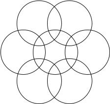
Figure 17.2 Three kinds of regions in the coverage of a base.

interesting range of R/r, there are three kinds of regions in which calls have potential access to one, two or three base stations. These regions in Figure 17.2 are denoted A1, A2 and A3, respectively. A1 is the nonoverlapping region while both A2 and A3 are overlapping regions. We consider (without loss of generality) the cell radius, r, to be normalized to unity. The coverage radius, R, is determined by the requirement of the link quality. Once R is found, the percentage of a cell that belongs to region A1, A2 or A3 can be calculated. They are denoted by p1, p2 and p3, respectively. These relationships are discussed letter in the section.

Reuse partitioning that has two partitions of channels, denoted a and b, is used. Systems with more partitions can be considered similarly. Channels of these two partitions are referred to as a- and b-type channels, respectively. These two partitions are used with different cluster sizes, Na and Nb, to allocate channels to base stations. Channels of type a are equally divided into Na groups each with Ca channels. Similarly, b-type channels are equally divided into Nb groups each with Cb channels. Every base station is assigned one group of channels from each partition in such a way that co-channel interference is minimized. As a result, there are totally Ca + Cb channels available at a base. Let CT denote the total number of available channels and f denote the fraction of channels that are assigned to partition a. So,

Since Na and Nb are different, Na is assumed to be the smaller one. Consequently a-type channels must be used in a smaller area. Channels of type a are intended for use by users who can access only one base, which corresponds to users in region A1. Channels of type b can be used by all users. Figure 17.3 shows the channel assignment and the available channel groups in a specific region for such a system with Na = 3 and Nb = 7. The three groups of a-type channels are labeled a1, a2 and a3, and the seven groups of b-type channels are labeled b1, b2, . . . , b7. Because of overlapping coverage, users in region A2 can access two groups of channels from partition b. Similarly, users in A3 can access three groups of b-type channels.

670 NETWORK DEPLOYMENT

Figure 17.3 The relationship between channel groups and various regions for Na = 3 and Nb = 7.

Priority to handoff calls is given at each base, by allocating Cha of the Ca a-type channels to handoffs. Similarly, Chb of the Cb b-type channels are reserved at a base. Specific channels are not reserved, only the numbers, Cha and Chb. As a result, new calls that arise in region A1 can access Ca − Cha a-type channels and Cb − Chb b-type channels at the corresponding base. New calls that arise in region A2 or A3 can access Cb − Chb channels of b-type at each potential base. New calls that arise in region A1 are served by b-type channels only when no a-type channel is available. When more than one base has a channel available to serve a new call that arises in region A2 or A3, the one with the best link quality is chosen. Most likely, it is the nearest one under uniform propagation and flat terrain conditions.

The possible types of handoffs are shown in Figure 17.3. The received signal power is inversely proportional to the distance raised to an exponent, γ , which is called path loss exponent. The coverage radius, R, is determined such that the worst case SIR of a-type calls is equal to the worst case SIR of b-type calls. Therefore, the desired R is the one that satisfies SIR a (R, Na , γ ) = SIR b(R, Nb, γ ). Mobile users are assumed to be uniformly distributed throughout the service area. Call arrivals follow a Poisson point process with a rate n per cell, and this rate is independent of the number of calls in progress. Session duration, T , is a random variable with a negative exponential probability density function

¯ = μ−1). An (or )-type call resides within the pertaining region during the with mean T ( a b

areas. Although region A1 is not circular, an equivalent radius (which is the radius of a circle that has the same area as A1) can be used. System modeling is based on using two variables to specify the state of a base. One is the number of a-type channels in use; the other is the number of b-type channels in use. A complete state representation for the whole system will be a string of base station states with two variables for each base. This

state representation can keep track of all events that occur in the system. Unfortunately, the huge number of system states precludes using this approach for most cases of interest. A simplified approach is to decouple a base from others using average teletraffic demands related to neighboring bases. This is similar to the approach used in References [13, 14]. As a result, the state, s, is characterized from a given base by a(s), b(s), where a(s) is the number of a-type channels in use in state s, and b(s) is the number of b-type channels in use in state s with constraint 0 ≤ a(s) ≤ Ca and 0 ≤ b(s) ≤ Cb. The state probabilities, P(s), in statistical equilibrium are needed for determining the performance measures of interest. To calculate state probabilities, the state transitions and the corresponding transition rates must be identified and calculated. Owing to overlapping coverage and reuse partitioning, state transitions result from six driving processes:

(1)new call arrivals;

(2)call completions;

(3)handoff departures of a type; calls that use a-type channels are a-type calls and those that use b-type channels are b-type calls. An a-type call initiates a handoff (a-type handoff) when it leaves region A1. An a-type handoff may be an inter-base or an intra-base handoff depending on which base continues its service (see Figure 17.3);

(4)hand-off arrivals of a type;

(5)handoff departures of b type; a b-type call initiates a handoff (b-type handoff) only when it leaves the coverage of the serving base. A b-type handoff that enters region A1 of a neighboring base (out of the coverage of the serving base) can access channels from both a-type and b-type (a-type channels first) at that target base. A b-type handoff that enters region A2 can access all channels of b-type at each potential target base; and

(6)hand-off arrivals of b type.

The transition rates from a current state s to next state sn due to these driving processes are denoted by rn (s, sn ), rc(s, sn ), rda (s, sn ), rha (s, sn ), rdb(s, sn ), and rhb(s, sn ), respectively. The details for state transition rate derivation and solving the system of state probabilities equations is based on the general principles discussed in Chapter 6. Some specific details can be found also in References [7, 8, 13, 14–16] and especially [17].

Td = 60 s, Cha = 0, Chb = 0 and γ = 4, are shown in Figures 17.4–17.6.

17.2 IMBEDDED MICROCELL IN CDMA MACROCELL NETWORK

Combining a macrocell and microcell with a two-tier overlaying and underlaying structure for a CDMA system is to become an increasingly popular trend in 4G wireless networks. However, the cochannel interference from a microcell to macrocell and vice versa in this two-tier structure is different from that in the homogeneous structure (i.e. consisting of only macrocells or only microcells).

674 NETWORK DEPLOYMENT

proportional to d2, otherwise, it is proportional to d4, where d is the distance away from the transmitter. The received power is represented as

where Pt is the power of the transmitter, hm and hb are the height of the mobile and BS antennas respectively, and bp is the breakpoint [17–20]. The MS will access a cell BS with the strongest pilot signal. After an MS determines to access a certain cell BS, the cell BS will verify whether or not the ratio for uplink signal to interference (C/I ) from a mobile is less than a threshold of (C/I )tu. If the C/I is less than the threshold of (C/I )tu, the MS is inhibited and blocked. In other words, for a call to be accepted we should have

where Pr j is the power received from the desired jth MS by a dedicated BS, Pt k is the power transmitted from the kth MS belonging to other BSs, and (β)k is the path loss from the kth MS to the dedicated BS. The first and second terms in the denominator represent the interference from other MSs in the same BS and from MSs belonging to other BSs, respectively. Thermal noise is rather small relative to the cells’ interference, so it is neglected. If Pr is increased, the interference from other cells is relatively smaller so that the C/I requirement for newly active users can be satisfied.

17.2.1 Macrocell and microcell link budget

For the handoff analysis we want to find the point where the strength of pilot signal emitted from a microcell BS is equal to that from a macrocell at the microcell boundary. The microcell boundary is assumed here to be distant from the macrocell bp. The distance from the microcell BS to the center of microcell is x. Therefore, the pilot power (emitted from microcell BS) received at boundary point D shown in Figure 17.7 is represented as

where αs is the power fraction of the pilot signal for microcells. Similarly, the pilot power received from the macrocell BS at boundary D is represented by

where αl is the ratio of pilot power to the BS’s downlink power and d1 is the distance between the centers of macrocells and microcells. The above equation is similar to (17.1). The subscripts xs (or xl) of Pxs (or Pxl) denote symbols for the microcell (small cell) or for the macrocell (large cell). Since the strengths of the pilot signals emitted from both the microcell BS and macrocell BS at D point are equal (i.e. PrsD = PrlD), the transmission

676 NETWORK DEPLOYMENT

x d

BS

Figure 17.8 Cell geometry for calculation of interference.

and

respectively, where Pr and Pr are mobile powers received by the macrocell’s BS and microcell’s BS, respectively, M and N denote the number of active mobiles in each microcell and macrocell, respectively. The first term and the second term in the denominator represent the interference from other MSs in the same BS and from all MSs in the other kind of BS, and ri and di are the distance from the ith mobile to its own BS and to the other kind of BS, respectively. Finally, the third term Ill (or Ils) represents the interference from adjacent macrocells to the central macrocell BS (or microcell BS). The above formulas are the decision rules for the uplink to accept a newly active MS. To find expression for Ill (or Ils), N mobile units are assumed to be uniformly distributed in an equivalent disc of radius R shown in Figure 17.8. The density of mobile unit is ρ = N /π R2 [1, 20].

The power received in the BS from each mobile is assumed here to be Pr with a path loss proportional to the fourth power of distance. The interference caused by mobiles in an adjacent macrocell is

√(d2 + r2 − 2dr cos θ ) is the distance between the mobile in the adjacent macrocell and

the interfered BS, and d is the distance between two BSs. Therefore, the interference to the central macrocell BS caused by the six adjacent macrocells can be calculated as

Similarly, the interference to the microcell BS caused by the six adjacent macrocells is expressed as

depending on the location of microcell.

17.2.2 Performance example

A detailed analysis of the above system by simulation is given in Wu et al. [20]. Four different power control schemes are analyzed:

(1)both the macrocell and microcell use the signal-strength-based power control for the uplink and there is no power control for the downlink;

(2)(a) [or scheme 2(b)], both the macrocells and microcells use the signal-strength- based power control for the uplink, and downlink power control is also applied for the microcell (or applied for macrocells and microcells);

(3)both the macrocells and microcells use the C/I power control for the uplink and there is no power control for the downlink;

(4)both the macrocells and microcells apply the C/I power control for uplink, however, but only the microcell uses power control for the downlink.

In addition, antenna heights of macrocells and microcells are 45 and 6 m, respectively. The radius of the microcell is r = 1000 m, the radius of the macrocell is R, and R = 10r. The bps are 342 m for the microcell and 2569 m for the macrocell.

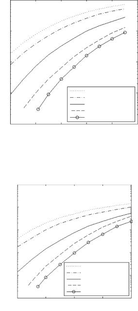
The arrival process for users in a cell is Poisson distributed with a mean arrival rate of λ, and the holding time for a call is exponentially distributed with the mean of 1/μ. The required Eb/N0 for uplink and downlink in a CDMA system is around 7 and 5 dB, respectively, if the bit error rate is less than 10−3. The major performance we are concerned with is the capacity. Under this maximum loading condition, the background noise is very little relative to interference, so that C/I is the only index to survey. The processing gain for a CDMA system is defined as the ratio of bandwidth over data rate, that is, 21.0 dB (i.e. 1.2288 MHz/9.6 kbs), so that the threshold of (C/I )tu is 14 dB for uplink and the threshold (C/I )td is 16 dB for the downlink.For this set of parameters the blocking probabilities for the two cells are given in Figures 17.9 and 17.10.

17.3 MULTITIER WIRELESS CELLULAR NETWORKS

In this section we further extend the previous problem to a general cell-design methodology in multitier wireless cellular network. Multitier networks may be a solution when there are a