

Advanced Wireless Networks - 4G Technologies
.pdf748 NETWORK INFORMATION THEORY
To prove the above results, consider bit b, where 1 ≤ b ≤ λnT . Let us suppose that it moves from its origin to its destination in a sequence of h(b) hops, where the hth hop traverses a distance of rbh . Then from (a3) we have
λnT h(b)
b |
¯ |
(19.39) |
rb |
≥ λnT L |
b=1 h=1
Having in mind that in any slot at most n/2 nodes can transmit for any subchannel m and any slot s we have
λnT h(b) |
Wm τ n |
|
1 (the hth hop of bit b is over subchannel m in slot s ) ≤ |
||
2 |
||
b=1 h=1 |
|
Summing over the subchannels and the slots, and noting that there can be no more than T/τ slots in T s yields
|
λnT |
WTn |
|
|
H : = |
h(b) ≤ |
(19.40) |
||
|
||||
2 |
||||
|
b=1 |
|
|
From the triangle inequality and (a6), for the protocol model, where X j is receiving a transmission from Xi over the mth subchannel and at the same time X is receiving a transmission from Xk over the same subchannel, we have
|X j − X | ≥ |X j − Xk | − |X − Xk | ≥ (1 + )|Xi − X j | − |X − Xk |
Similarly,
|X − X j | ≥ (1 + )|Xk − X | − |X j − Xi |
Adding the two inequalities, we obtain
|X − X j | ≥ |
|
(|Xk − X | + |Xi − X j |) |
2 |
This means that disks of radius /2 times the lengths of hops centered at the receivers over the same subchannel in the same slot are essentially disjoint. This conclusion also directly follows from the alternative restriction in (a6). Allowing for edge effects where a node is near the periphery of the domain, and noting that a range greater than the diameter of the domain is unnecessary, we see that at least a quarter of such a disk is within the domain. Having in mind that at most Wm τ bits can be carried in slot from a receiver to a transmitter over the mth subchannel, we have
λnT h(b) |
1 |
|
|
2 |
|
1 (the hth hop of bit b is over subchannel m in slot s)× |
π |
(rbh )2≤Wm τ |
|||
|
|
||||
4 |
2 |
||||
b=1 h=1 |
|
|
|
|
(19.41)
Summing over the subchannels and the slots gives
λnT h(b) |
π 2 |
|
|
|
(rbh )2 ≤ W T |
b=1 h=1 |
16 |
|
|
|
|

CAPACITY OF AD HOC NETWORKS |
749 |
or equivalently
λnT h(b) |
1 |
(rbh )2 ≤ |
16WT |
(19.42) |
|
|
|
||
b=1 h=1 |
H |
π 2 H |
||
|
|
|
|
Since the quadratic function is convex we have
λnT h(b) |
2 |
λnT h(b) 1 |
|
|
|
||
1 |
rbh ≤ |
rbh |
2 |
(19.43) |
|||
b=1 h=1 |
H |
b=1 h=1 |
H |
|
|||
|
|
|
|
|
|
||
Finally combining Equations (19.64) and (19.65) yields
λnT h(b) |
|
16WTH |
|
|
rbh ≤ |
|
(19.44) |
||
|
|
|
||
|
π 2 |
|||
b=1 b=1 |
|
|
|
|
and substituting Equation (19.40) in Equation (19.66) gives
¯ |
16WTH |
|
|
λnT L ≤ |
|
|
(19.45) |
π 2 |
|||
Substituting Equation (19.63) in Equation (19.67) yields the result (r1).
For the physical model suppose Xi is transmitting to X j(i) over the mth subchannel at power level Pi at some time, and let denote the set of all simultaneous transmitters over the mth subchannel at that time. The initial constraint introduced by (a6) can be represented as
S |
|
|
Pi |
|
|
|
||
|Xi −X j | |
|
|
||||||
|
= |
|
|
α |
≥ β |
(19.46) |
||
I |
N + k |
Pk |
||||||
|
|
|Xk − X j |α |
|
|
|
|||
k =i
By also including the signal power of Xi in the denominator, the signal-to-interference
requirement for X j(i) |
can be written as |
|
|
|
|
|
|
|
|
|
|
|
|
|
|||||||||||||||||
|
|
|
|
|
|
|
|
|
|
S |
|
|
|
|
|
Pi |
|
|
|
|
|
|
|
β |
|
|
|
||||
|
|
|
|
|
|
|
|
|
|
|
|
|Xi −X j(i)| |
α |
|
|
|
|
|
|||||||||||||
|
|
|
|
|
|
|
|
|
|
|
|
= |
|
|
|
|
|
|
|
≥ |
|
|
|
|
|||||||
|
|
|
|
|
|
|
|
|
|
I |
|
N |
+ k |
|
|
Pk |
|
β + 1 |
|
||||||||||||
|
|
|
|
|
|
|
|
|
|
|
|
|
|
|
|
|
|Xk − X j(i)|α |
||||||||||||||
|
|
|
|
|
|
|
|
|
|
|
|
|
|
|
|
|
|
|
|
|
|
|
|
||||||||
which results in |
|
|
|
|
|
|
|
|
|
|
|
|
|
|
|
|
|
|
|
|
|
|
|
|
|
|
|
||||
|
| |
X |
i − |
X |
j(i)| |
α |
≤ |
β + 1 |
|
|
|
|
|
|
Pi |
|
|
|
|
|
≤ |
β + 1 |
|
|
Pi |
||||||
|
|
|
|
|
β |
N |
+ k |
|
Pk |
|
|
|
β |
|
N + ( π4 )α/2 Pk |
||||||||||||||||
|
|
|
|
|
|
|
|
|
|
|
|
|
|
|
|Xk − X j(i)|α |
|
|
|
|||||||||||||
|
|
|
|
|
|
|
|
|
|
|
|
|
|
|
|
|
|
|
|
|
|
k |
|||||||||
(since |
|Xk − X j(i)| ≤ |
2/√ |
|
|
). |
|
|
|
|
|
|
|
|
|
|
|
|
|
|
|
|
|
|||||||||
|
|
|
|
|
|
|
π |
|
|
|
|
|
|
|
|
|
|
|
|
|
|
|
|
|
|||||||

750 NETWORK INFORMATION THEORY
Summing over all transmitter–receiver pairs,
|
|
|
|
|
|
|
β + 1 |
|
|
|
Pi |
|
|
|
|
|
β + 1 |
i | |
X |
i − |
X |
j(i)| |
α |
≤ |
|
|
i |
|
≤ |
2α |
π −(α/2) |
||||
|
β N + ( π4 )α/2 |
Pk |
β |
||||||||||||||
|
|
|
|
|
|||||||||||||
|
|
|
|
|
|
|
|
|
|
|
i |
|
|
|
|
|
|
Summing over all slots and subchannels gives |
|
|
|
|
|
|
|
||||||||||
|
|
|
|
λnT h(b) |
|
|
|
|
π − α2 |
β + 1 |
|
|
|
|
|||
|
|
|
|
|
|
|
rα (h, b) |
≤ |
2α |
W T |
|
|
|||||
|
|
|
|
|
|
|
|
|
|
||||||||
|
|
|
|
b=1 h=1 |
|
|
β |
|
|
|
|
|
|||||
|
|
|
|
|
|
|
|
|
|
|
|
|
|||||
The rest of the proof proceeds along lines similar to the protocol model, invoking the convexity of rα instead of r2. For the consideration of the special case where Pmax/ Pmin < β, we start with Equation (19.46). From it, it follows that if Xi is transmitting to X j at the same time that Xk is transmitting to X , both over the same subchannel, then
|
Pi |
|
|
|
|Xi −X j |α |
|
≥ β |
|
Pk |
|
|
|
|Xk −X j |α |
|
|
Thus
1
|Xk − X j | ≥ (β Pmin/ Pmax) α |Xi − X j | = (1 + )|Xi − X j |
1
where := (β Pmin/ Pmax) α − 1. Thus the same upper bound as for the protocol model carries over with defined as above.
19.2.4 Arbitrary networks: lower bound on transport capacity
There is a placement of nodes and an assignment of traffic patterns such that the network
can achieve |
|
|
|
|
|
|
|
|
|
|
|
|
|
|
||
|
|
|
|
|
√ |
|
|
|
√ |
|
|
|
|
|
|
|
|
|
|
|
|
|
|
|
|
|
|
|
|
||||
W n/ (1 + 2 ) |
n + |
|
8π |
|
|
b-m/s |
||||||||||
under the protocol model, |
|
|
|
|
|
|
|
|
|
|
|
|
|
|
||
|
|
|
|
|
|
|
|
α |
|
|
|
α |
2 |
|
−1/α |
|
√ |
|
|
√ |
|
|
|
|
6 |
|
− |
|
|
||||
|
|
2 |
2 |
+ |
|
|
|
b-m/s |
||||||||
W n/ n + |
|
8π 16β |
|
|
α |
− |
2 |
|||||||||
|
|
|
|
|
|
|
|
|
|
|
|
|
|
|
||
under the physical model, both whenever n is a multiple of 4. To prove it, consider the protocol model and define
√
r := 1/ (1 + 2 ) n/4 + 2π
Recall that the domain is a disk of unit area, i.e. of radius 1/√π in the plane. With the center of the disk located at the origin, place transmitters at locations [ j(1 + 2 )r ± r, k(1 + 2 )r] and [ j(1 + 2 )r, k(1 + 2 )r ± r] where | j + k| is even. Also place receivers at [ j(1 + 2 )r ± r, k(1 + 2 )r] and [ j(1 + 2 )r, k(1 + 2 )r ± r] where | j + k| is odd. Each transmitter can transmit to its nearest receiver, which is at a distance r away, without interference from any other transmitter–receiver pair. It can be verified that there are at

CAPACITY OF AD HOC NETWORKS |
751 |
least n/2 transmitter–receiver pairs, all located within the domain. This is based on the fact that for a tessellation of the plane by squares of side s, all squares intersecting a disk of radius R − √2s are entirely contained within a larger concentric disk of radius R. The number of such squares is greater than π (R − √2s)2/s2. This proves the above statement for s = (1 + 2 )r and R = 1/√π . Restricting attention to just these pairs, there are a total of n/2 simultaneous transmissions, each of range r, and each at W b/s. This achieves the transport capacity indicated.
For the physical model, a calculation of the SIR shows that it is lower-bounded at all receivers by
(1 + 2 )α |
α |
|
6α−2 −1 |
|||
16 2 2 |
+ |
|
|
|
|
|
α |
− |
2 |
||||
|
|
|
|
|
|
|
Choosing to make this lower bound equal to β yields the result.
In the protocol model, there is a placement of nodes and an assignment of traffic patterns
such that the network can achieve |
|
|||||||||||||
2W/√ |
|
|
|
b-m/s for n ≥ 2 |
|
|||||||||
π |
|
|||||||||||||
4W |
√ |
|
(1 + ) −1 b-m/s, for n ≥ 8 |
|
||||||||||
π |
|
|||||||||||||
W n |
(1 + 2 ) √ |
|
+ √ |
|
|
−1 |
|
|||||||
|
8π |
|
b-m/s, for n = 2, 3, 4, · · · , 19, 20, 21 and |
|||||||||||
n |
||||||||||||||
4 n/4 W (1 + 2 ) |
√ |
|
|
+ √ |
|
−1 |
||||||||
4 n/4 |
8π |
b-m/s, for all n |
||||||||||||
With at least two nodes, clearly 2W/√π b-m/s can be achieved by placing two nodes at diametrically opposite locations. This verifies the formula for the bound for n ≤ 8. With at least eight nodes, four transmitters can be placed at the opposite ends of perpendicular diameters,
and each can transmit toward its receiver located at a distance 1/ |
√ |
|
(2 |
+ |
2 ) towards |
|||||||
π |
|
|||||||||||
the center of the domain. This yields 4 |
W |
/ |
√ |
|
(1 |
+ |
) b-m/s, verifying the formula up to |
|||||
|
π |
|
||||||||||
n = 21. |
|
|
|
|
|
|
|
|
|
|
|
|
19.2.5 Random networks: lower bound on throughput capacity
In this section we show that one can spatially and temporally schedule transmissions in a random graph so that, when each randomly located node has a randomly chosen destination, each source–destination pair can indeed be guaranteed a ‘virtual channel’ of capacity cW (1 + )2√n log n −1 b/s with probability approaching 1 as n → ∞, for an appropriate constant c > 0. We will show how to route traffic efficiently through the random graph so that no node is overloaded.
19.2.5.1 Spatial tessellation
In the following a Voronoi tessellation of the surface S2 of the sphere is used. For a set of p points {a1, a2, · · · , ap } on S2 the Voronoi cell V (ai ) is the set of all points which are closer to ai than to any of the other a j s, i.e. [34],
V (ai ) := {x S2 : |x − ai | = min |x − a j |}
1≤ j≤ p

752 NETWORK INFORMATION THEORY
D (x, 2e)
D (x, e)
Figure 19.7 A tessellation of the surface S2 of the sphere.
Above and throughout, distances are measured on the surface S2 of the sphere by segments of great circles connecting two points. The point ai is called the generator of the Voronoi cell V (ai ). The surface of the sphere does not allow any regular tessellation where all cells look the same. For our application Voronoi tessellations will also need to be not too eccentrically shaped. Therefore, the properties of Voronoi tessellations needed in this section can be summarized as:
(v1) For every ε > 0, there is a Voronoi tessellation of S2 with the property that every Voronoi cell contains a disk of radius ε and is contained in a disk of radius 2ε (see illustration in Figure 19.7).
To prove this we denote by D(x, ε) a disk of radius ε centered at x. Choose a1 as any point in S2. Suppose that a1, · · · , ap have already been chosen such that the distance between any two a j s is at least 2ε. There are two cases to consider. Suppose there is a point x such that D(x, ε) does not intersect any D(ai , ε). Then x can be added to the collection: Define ap+1 := x. Otherwise, we stop. This procedure has to terminate in a finite number of steps since the addition of each ai removes the area of a disk of radius ε > 0 from S2. When we stop we will have a set of generators such that they are at least 2ε units apart, and such that all other points on S2 are within a distance of 2ε from one of the generators. The Voronoi tessellation obtained in this way has the desired properties.
In the sequel we will use a Voronoi tessellation Vn for which
(v2) Every Voronoi cell contains a disk of area 100 log n/n.
Let ρ(n) := radius of a disk of area (100 log n) /n on S2.
(v3) Every Voronoi cell is contained in a disk of radius 2ρ(n).
We will refer to each Voronoi cell V Vn as simply a ‘cell’.
CAPACITY OF AD HOC NETWORKS |
753 |
19.2.5.2 Adjacency and interference
By definition, two cells are adjacent, if they share a common point. If we choose the range r(n) of each transmission so that r(n) = 8ρ(n), this range will allow direct communication within a cell and between adjacent cells.
(v4) Every node in a cell is within a distance r(n) from every node in its own cell or adjacent cell.
To prove it let we notice that the diameter of cells is bounded by 4ρ(n), see (v3). The range of a transmission is 8ρ(n). Thus the area covered by the transmission of a node includes adjacent cells.
19.2.5.3 Interfering neighbors
By definition we say that two cells are interfering neighbors if there is a point in one cell which is within a distance (2 + )r(n) of some point in the other cell. In other words if two cells are not interfering neighbors, then in the protocol model a transmission from one cell cannot collide with a transmission from the other cell.
19.2.5.4 Bound on the number of interfering neighbors of a cell
An important property of the constructed Voronoi tessellation Vn is that the number of interfering neighbors of a cell is uniformly bounded. This will be exploited in the next section in constructing a spatial transmission schedule which allows for a high degree of spatial concurrency and thus frequency reuse.
(v5) Every cell in Vn has no more than c1 interfering neighbors were c1 depends only on and grows no faster than linearly in (1 + )2.
To prove it, Let V be a Voronoi cell. If V is an interfering neighboring Voronoi cell, there must be two points, one in V and the other in V , which are no more than (2 + )r(n) units apart. From (v3), the diameter of a cell is bounded by 4ρ(n). Hence V , and similarly every other interfering neighbor in the protocol model, must be contained within a common
large disk D of |
radius 6ρ( |
) |
+ |
(2 |
+ |
) ( |
n |
). Such a disk |
D |
cannot contain more than |
||
|
2 |
n2 |
|
|
r |
|
|
|||||
c2{[6ρ(n) + (2+ =)r(n)] /ρ |
(n)} disks of radius ρ(n). From (v2), there can therefore be |
|||||||||||
no more than this number of cells within D. This then is an upper bound on the number of interfering neighbors of the cell V . The result follows from the chosen magnitudes of ρ(n) and r(n).
19.2.5.5 A bound on the length of an all-cell inclusive transmission schedule
The bounded number of interfering neighbors for each cell allows the construction of a schedule of bounded length which allows one opportunity for each cell in the tessellation Vn to transmit.
(v6) In the Protocol Model there is a schedule for transmitting packets such that in every (1 + c1) slots, each cell in the tessellation Vn gets one slot in which to transmit, and such that all transmissions are successfully received within a distance r(n) from their transmitters.
754 NETWORK INFORMATION THEORY
(v7) There is a deterministic constant c not depending on n, N, α, β, or W such that ifis chosen to satisfy
1 2
(1 + )2 > 2 cβ 3 + (α − 1)−1 + 2 (α − 2)−1 α − 1
then for a large enough common power level P, the above result (v6) holds even for the physical model.
To prove it we show first the result for the protocol model. This follows from a well-known fact about vertex coloring of graphs of bounded degree. A graph of degree no more than c1 can have its vertices colored by using no more than (1 + c1) colors, with no two neighboring vertices having the same color [35]. One can therefore color the cells with no more than (1 + c1) colors such that no two interfering neighbors have the same color. This gives a schedule of length at most (1 + c1), where one can transmit one packet from each cell of the same color in a slot.
For the physical model one can show that, under the same schedule as above, the required SIR of β is obtained if each transmitter chooses an identical power level P that is high enough, and is large enough. From the previous discussion we know that any two nodes transmitting simultaneously are separated by a distance of at least (2 + )r(n) and disks of radius (1 + /2)r(n) around each transmitter are disjoint. The area of each such disk is at least c3π (1 + /2)2r2(n). (In the case of disks on the plane c3 = 1, but it is smaller for disks on the surface of the sphere.)
Consider a node Xi transmitting to a node X j at a distance less than r(n). The signal power received at X j is at least Pr−α (n). Now we look at the interference power due to all the other simultaneous transmissions. Consider the annulus of all points lying within a distance between a and b from X j . A transmitter within this annulus has the disk centered at itself and of radius (1 + /2)r(n) entirely contained within a larger annulus of all points lying between a distance a − (1 + /2)r(n) and b + (1 + /2)r(n). The area of this larger annulus is no more than
c4π [b + (1 + /2) r(n)]2 − [a − (1 + /2) r(n)]2
Each transmitter above ‘consumes’ an area of at least c3π (1 + /2)2 r2(n), as noted earlier. Hence the annulus of points at a distance between a and b from the receiver X j cannot contain more than
|
|
|
|
|
|
|
|
−1 |
|||
c4π {[b + (1 + |
|
|
)r(n)]2 − [a − (1 |
+ |
|
)r(n)]2} |
c3π (1 + |
|
|
)2r2(n) |
|
|
2 |
2 |
2 |
|
|||||||
transmitters. Also, the received power at X j from each such transmission is at most P/aα . Noting that there can be no other simultaneous transmitter within a distance (1 + )r(n)
of X j , and taking a = k(1 + /2)r(n) and b = (k + 1)(1 + 2 )r(n) for k = 1 , 2 , 3, · · · , we see that the SIR at X j is lower-bounded by
|
|
|
|
+∞ |
|
|
|
|
|
|
|
|
|
|
|
|
|
|
−1 |
||
α |
|
|
|
|
|
2 |
|
|
|
2 |
|
α |
|
|
α α |
−1 |
|||||
Pr− |
(n) |
N + c4 P |
(k + 2) |
|
|
− (k − 1) |
|
c3k |
(1 |
+ |
|
) r |
(n) |
||||||||
|
|
|
2 |
||||||||||||||||||
|
|
|
|
k=1 |
|
|
|
|
|
|
|
|
|
−1 |
|
|
|
|
|||
|
|
P |
|
rα (n) |
|
|
|
c4 |
|
|
P |
+∞ |
6k + 3 |
|
|
|
|
||||
|
|
|
|
|
|
|
|
|
|
|
|
|
|||||||||
= |
|
|
|
+ c3 |
|
|
|
|
|
|
|
|
|
|
|
||||||
|
N |
|
(1 |
+ /2)α N k=1 kα |
|
|
|
|
|
|
|
||||||||||

INFORMATION THEORY AND NETWORK ARCHITECTURES |
755 |
Since α > 2, the sum in the denominator converges, and is smaller than 9 + 3 (α − 1)−1 + 6 (α − 2)−1. When is as specified and P → ∞, the lower bound on the SIR converges to a value greater than β. Using similar arguments one can show that [32]
(v8) Each cell contains at least one node.
(v9) The mean number of routes served by each cell ≤ c10√(n log n). (v10) The actual traffic served by each cell ≤ c5λ(n)√(n log n whp).
19.2.5.6 Lower bound on throughput capacity of random networks
From (v6) we know that there exists a schedule for transmitting packets such that in every (1 + c1) slots, each cell in the tessellation Vn gets one slot to transmit, and such that each transmission is received within a range r(n) of the transmitter. Thus the rate at which each cell gets to transmit is W/(1 + c1) b/s. On the other hand, the rate at which each cell needs to transmit is with high probability (whp) less than c5λ(n)√n log n [see (v10)]. With high probability, this rate can be accommodated by all cells if it is less than the rate available, i.e. if c5λ(n)√(n log n) ≤ W (1 + c1)−1. Moreover, within a cell, the traffic to be handled by the entire cell can be handled by any one node in the cell, since each node can transmit at rate W b/s whenever necessary. In fact, one can even designate one node in each cell as a ‘relay’ node. This node can handle all the traffic needing to be relayed. The other nodes can simply serve as sources or sinks.
We have proved the following theorem, noting the linear growth of c1 in (1 + )2 in (v5), and the choice of in (v6) for the physical model.
(v11) For random networks on S2 in the protocol model, there is a deterministic constant c > 0 not depending on n, , or W, such that λ(n) = cW (1 + )2√(n log n) −1 b/s is feasible whp.
(v12) For random networks on S2 in the physical model, there are deterministic constants c and c not depending on n, N, α, β, or W, such that
1 2
λ(n) = c W 2 c β 3 + (α − 1)−1 + 2 (α − 2)−1 α − 1 n log n b/s
is feasible whp. These throughput levels have been attained without subdividing the wireless channel into subchannels of smaller capacity.
19.3 INFORMATION THEORY AND NETWORK ARCHITECTURES
19.3.1 Network architecture
For the optimization of ad hoc and sensor networks we will discuss some performance measure for the architectures shown in Figures 19.8–19.11. We will mainly focus on trans-
port capacity CT := sup m Rl ρl , where the supremum is taken over m, and vectors
l=1
(R1, R2, . . . , Rm ) of feasible rates for m source-destination pairs, and ρl is the distance

756 NETWORK INFORMATION THEORY
j
ρij rmin
 i
i
Figure 19.8 A planar network: n nodes located on a two-dimensional plane, with minimum separation distance ρmin.
(1, n ) (2, n ) |
( n, n) |
(1,1) (2,1) |
( n, 1) |
Figure 19.9 A regular planar network: n nodes located on a plane at (i, j) with 1 ≤ i, j ≤ √n. (Reproduced by permission of IEEE [33].)
between the lth source and its destination. For the planar network from Figure 19.8 we assume [33]:
(1)There is a finite set N of n nodes located on a plane.
(2)There is a minimum positive separation distance ρmin between nodes, i.e. ρmin :=
mini=j ρi j > 0, where ρi j is the distance between nodes i, j N .
(3)Every node has a receiver and a transmitter. At time instants t = 1, 2, . . . , node i N sends Xi (t), and receives Yi (t) with
Yi (t) = |
|
eγρi j X j (t) |
+ Zi (t) |
j=i |
ρiδj |
||
|
|
|
where Zi (t), i N, t = 1, 2, . . . are Gaussian independent and identically distributed (i.i.d.) random variables with mean zero and variance σ 2. The constant δ > 0 is referred to as the path loss exponent, while γ ≥ 0 will be called the
INFORMATION THEORY AND NETWORK ARCHITECTURES |
757 |
|
rij |
rmin |
|
i |
j |
|
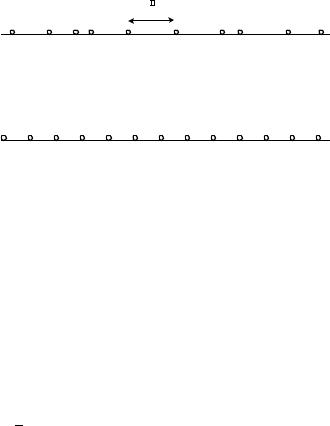
Figure 19.10 A linear network: n nodes located on a line, with minimum separation distance ρmin. (Reproduced by permission of IEEE [33].)
1 |
2 |
i i + 1 |
n |
Figure 19.11 A regular linear network: n nodes located on a line at 1, 2, . . . , n. (Reproduced by permission of IEEE [33].)
absorption constant. A positive γ generally prevails except for transmission in a vacuum, and corresponds to a loss of 20γ log10 e decibel per meter.
(4) Denote by |
Pi ≥ 0 |
the power used by node i. Two |
separate |
constraints on |
||
|
|
n |
|
|||
{ P1, P2, . . . , Pn } are studied: total power constraint Ptotal : |
i=1 |
Pi ≤ Ptotal or in- |
||||
dividual power constraint Pind : Pi ≤ Pind, for i = 1, 2, . . . , n.
(5) The network can have several source–destination pairs (s , d ), = 1, . . . , m, where s , d are nodes in N with s =d , and (s , d ) =(s j , d j ) for =j. If m = 1, then there is only a single source–destination pair, which we will simply denote (s, d).
A special case is a regular planar network where the n nodes are located at the points (i, j) for 1 ≤ i, j ≤ √n; see Figure 19.9. This setting will be used mainly to exhibit achievability of some capacities, i.e. inner bounds. Another special case is a linear network where the n nodes are located on a straight line, again with minimum separation distance ρmin; see Figure 19.10. The main reason for considering linear networks is that the proofs are easier to state and comprehend than in the planar case, and can be generalized to the planar case. Also, the linear case may have some utility for, say, networks of cars on a highway, since its scaling laws are different.
A special case of a linear network is a regular linear network where the n nodes are located at the positions 1, 2, . . . , n; see Figure 19.11. This setting will also be used mainly to exhibit achievability results.
19.3.2 Definition of feasible rate vectors
Definition 1
Consider a wireless network with multiple source–destination pairs (s , d ), = 1, . . . , m, with s =d , and (s , d ) =(s j , d j ) for =j. Let S := {s , = 1, . . . , m} denote the set of source nodes. The number of nodes in S may be less than m, since we allow a node