Advanced Wireless Networks - 4G Technologies

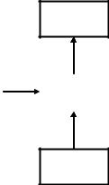
Figure 16.9 Mobile terminal architecture.

hardware or as a kernel module of common operating systems. The forwarding engine is programmable for performance-critical tasks which are performed on a per-packet basis.

The interface modules are medium specific for different wireless or wired standards. They can be configured or programmed to adapt to new physical layer protocols or for triggering events in higher layers.

There are different approaches to active networking in this architecture. Some approaches offer a virtual execution environment, e.g. a Java virtual machine, on the middleware layer. Some options also include native code in the computing platform, e.g. for flexible signaling. Others employ programmable hardware for forwarding.

A key ingredient in these approaches is interfaces to the lower layers and programmable filters for identifying the packets to be processed in the active networking environment. The terminal architecture is shown in Figure 16.9. It consists of:

Middleware platform, typically with a limited virtual execution environment.

Smart Card, e.g. USIM for UMTS, which includes subscriber identities and also a small, but highly secure execution environment. This can be used ideally for personal services like electronic wallet.

Programmable hardware, which is designed for one or more radio standards.

Native operating system which provides real-time support, needed for stacks and certain critical applications, e.g. multimedia codecs.

Compared with network elements, the SmartCard is a new, programmable component. Owing to resource limitations, the forwarding engine and computation platform just collapse to one operating system platform. Also, the middleware layers are typically quite restricted. Service deployment and control of reconfigurations are complex since there is a split of responsibility between operator and manufacturer. For instance, the manufacturer has to provide or digitally sign appropriate low-level code for reconfigurations. On the other hand, the operator is interested in controlling the configuration to fit the user and network needs.

There are a number of examples to show the importance of flexible networking protocols and the need of dynamic cross layer interfaces in future mobile networks. As an example we show that hand-over can be optimized by information about the user context [37, 42, 43]

640 ACTIVE NETWORKS

Train

AP3

Figure 16.10 Context-aware hand-over prediction.

as shown in Figure 16.10. In this scenario, the terminal moves into an area covered by both AP2 and AP3. The problem is to decide which access point (AP) to choose. State of the art are many algorithms based on signal strength analysis or on available radio resources. Even if one AP is slightly better regarding these local measurements, the decision may not be the best. For instance, if the terminal in Figure 16.10 is on the train, it is obviously better to hand over to AP3, even if AP2 is more reachable for a short period of time. In many cases, the hand-over can be optimized by knowledge of terminal movement and user preferences. For instance, if the terminal is in a car or train, its route may be constrained to certain areas. Also, the terminal profile may contain the information that the terminal is built in a car. Alternatively, the movement pattern of a terminal may suggest that the user is in a train. A main problem is that hand-over decisions have to be executed fast. However, the terminal profile and location information is often available on a central server in the core network. Retrieving this information may be too slow for hand-over decisions.

Furthermore, the radio conditions during hand-over may be poor and hence limit such information exchange. The idea of the solution is to proactively deploy a context-aware decision algorithm onto the terminal which can be used to assist hand-over decisions. A typical example is the information about the current movement pattern, e.g. by knowledge of train or road routes. For implementation, different algorithms can be deployed by the network on the terminal, depending on the context information. This implementation needs a cross layer interface, which collects the context information from different layers and makes an optimized decision about deploying a decision algorithm.

16.5 COGNITIVE PACKET NETWORKS

We now discuss packet switching networks in which intelligence is incorporated into the packets, rather than at the nodes or in the protocols. Networks which contain such packets are referred to as cognitive packet networks (CPN). Cognitive packets in CPN route themselves, and learn to avoid congestion and being lost or destroyed. Cognitive packets learn from their own observations about the network and from the experience of other packets. They rely

Figure 16.11 Format of cognitive packet.

Updated cognitive map

Cognitive map (CM)

Figure 16.12 CP update by a CPN node.

minimally on routers. Each cognitive packet progressively refines its own model of the network as it travels through the network, and uses the model to make routing decisions. Cognitive packets (CPs) store information in their private cognitive map (CM) and update the CM and make their routing decisions using the code which is in each packet. This code may include neural networks or other adaptive algorithms. Figure 16.11 presents the format of a cognitive packet. The manner in which cognitive memory at a node is updated by the node’s processor is shown in Figure 16.12. In a CPN, the packets use nodes as ‘rented space’, where they make decisions about their routes. They also use nodes as places where they can read their mailboxes. Mailboxes may be filled by the node, or by other packets which pass through the node. Packets also use nodes as processors which execute their code to update their CM and then execute their routing decisions. As a result of code execution, certain information may be moved from the CP to certain mailboxes. The nodes may execute the code of CPs in some order of priority between classes of CPs, for instance as a function of QoS requirements which are contained in the identification field).

As a routing decision, a CP will be placed in some output queue, in some order of priority, determined by the CP code execution. A CPN and a CPN node are schematically represented in Figures 16.13 and 16.14. CPs use units of information ‘signals’ to communicate with each other via mailboxes (MBs) in the nodes. These signals can also emanate from the environment (nodes, existing end-to-end protocols) toward the CPs. CP, shown in Figure 16.11, contain the following fields [44]:

(1)The identifier field (IF), which provides a unique identifier for the CP, as well as information about the class of packets it may belong to, such as its quality of service (QoS) requirements.

642 ACTIVE NETWORKS

Output

Processor

Input

CP

MB

A node

Mailboxes

Figure 16.13 CPN node model.

H

Cognitive packet network

Figure 16.14 CPN example.

(2)The data field containing the ordinary data it is transporting.

(3)A cognitive map (CM), which contains the usual source and destination (S-D) information, as well as a map showing where the packet currently ‘thinks’ it is, the packet’s view of the state of the network, and information about where it wants to go next; the S-D information may also be stored in the IF.

(4)Executable code that the CP uses to update its CM. This code will contain learning algorithms for updating the CM, and decision algorithms which use the CM.

A node in the CPN provides a storage area for CPs and for mailboxes which are used to exchange data between CPs, and between CPs and the node. It has an input buffer for CPs arriving from the input links, a set of mailboxes, and a set of output buffers which are associated with output links. Nodes in a CPN carry out the following functions [44]:

(1)A node receives packets via a finite set of ports and stores them in an input buffer.

(2)It transmits packets to other nodes via a set of output buffers. Once a CP is placed in an output buffer, it is transmitted to another destination node with some priority indicated in the output buffer.

(3)A node receives information from CPs which it stores in MBs. MBs may be reserved for certain classes of CPs, or may be specialized by classes of CPs . For instance, there may be different MBs for packets identified by different source-destination (S-D) pairs.

(4)A node executes the code for each CP in the input buffer. During the execution of the CPs code, the CP may ask the node to decline its identity, and to provide information about its local connectivity (i.e. this is node A, and I am connected to nodes B, C, D via output buffers) while executing its code. In some cases, the CP may already have this information in its CM as a result of the initial information it received at its source, and as a result of its own memory of the sequence of moves it has made.

As a result of this execution:

(1)The CMs of the packets in the input buffer are updated.

(2)Certain information is moved from CPs to certain MBs.

(3)A CP which has made the decision to be moved to an output buffer is transfered there, with the priority it may have requested.

We have been already discussing some networks which offer users the capability of adding network executable code to their packets. Additional material can be found in References [44–68].

16.5.1 Adaptation by cognitive packets

Each cognitive packet starts with an initial representation of the network from which it then progressively constructs its own cognitive map of the network state and uses it to make routing decisions. Learning paradigms are used by CPs to update their CM and reach decisions using the packet’s prior experience and the input provided via mailboxes. In the adaptive approach for CPs, each packet entering the network is assigned a goal before it enters the network, and the CP uses the goal to determine its course of action each time it has to make a decision [44]. For instance if the CP contains part of a telephone conversation, a typical goal assigned to the packet should reflect the concern about the delay. A more sophisticated goal in this case could be delay and sequenced (in order) delivery. On the other hand, if these were data packets, the goal may simply be packet loss rate. These goals are translated into numerical quantities (e.g. delay values, loss probabilities and weighted combinations of such numerical quantities), which are then used directly in the adaptation.

644 ACTIVE NETWORKS

An example is where all the packets were assigned a common goal, which was to minimize a weighted combination of delay (W ) and loss (L) as

A simple approach to adaptation is to respond in the sense of the most recently available data. Here the CP’s cognitive memory contains data which is updated from the contents of the node’s mailbox. After this update is made, the CP makes the decision which is most advantageous (lowest cost or highest reward) simply based on this information. This approach is referred to as the Bang-Bang algorithm. Instead some other learning paradigms for CPs can be also used like learning feedforward random neural networks (LFRNN) [57, 68] or random neural networks with reinforcement learning (RNNRL) [57]. Adaptive stochastic finite-state machines (ASFSM) [55, 56, 58] are another class of adaptive models which could be used for these purposes.

16.5.2 The random neural networks-based algorithms

For the reinforcement learning approach to CP adaptation, as well the feed-forward neural network predictor, the RNN [57] was used in Gelenbe et al. [44]. IT is an analytically tractable model whose mathematical structure is akin to that of queueing networks. It has product form just like many useful queueing network models, although it is based on nonlinear mathematics. The state qi of the ith neuron in the network is the probability that it is excited. Each neuron i is associated with a distinct outgoing link at a node. These quantities satisfy the following system of nonlinear equations:

Here wi+j is the rate at which neuron i sends ‘excitation spikes’ to neuron j when i is excited, and wi−j is the rate at which neuron i sends “inhibition spikes” to neuron j when i is excited and r(i) is the total firing rate from the neuron i. For an n neuron network, the network parameters are these n by n ‘weight matrices’ W+ = wi+j and W− = wi−j which need to be ‘learned’ from input data. Various techniques for learning may be applied to the RNN. These include reinforcement learning and gradient-based learning, which are used in the following.

Given some goal G that the CP has to achieve as a function to be to be minimized [i.e. transit delay or probability of loss, or a weighted combination of the two as in Equation (16.1)], a reward R is formulated which is simply R = 1/G. Successive measured values of the R are denoted by Rl, l = 1, 2, . . . These are first used to compute a decision threshold:

where a is some constant 0 < a < 1, typically close to 1. Now an RNN with (at least) as many nodes as the decision outcomes is constructed. Let the neurons be numbered 1, . . . , n.

Thus for any decision i, there is some neuron i. Decisions in this RL algorithm with the RNN are taken by selecting the decision j for which the corresponding neuron is the most excited, i.e. the one with has the largest value of q j . Note that the lth decision may not have contributed directly to the lth observed reward because of time delays between cause and effect. Suppose that we have now taken the lth decision which corresponds to neuron j, and that we have measured the lth reward Rl. Let us denote by ri the firing rates of the neurons before the update takes place. We first determine whether the most recent value of the reward is larger than the previous ‘smoothed’ value of the reward, which is referred to as the threshold Tl−1. If that is the case, then we increase very significantly the excitatory weights going into the neuron that was the previous winner (in order to reward it for its new success), and make a small increase of the inhibitory weights leading to other neurons. If the new reward is not better than the previously observed smoothed reward (the threshold), then we simply increase moderately all excitatory weights leading to all neurons, except for the previous winner, and increase significantly the inhibitory weights leading to the previous winning neuron (in order to punish it for not being very successful this time). This is detailed in the algorithm given below. We compute Tl−1 and then update the network weights as follows for all neurons i =j:

Then we re-normalize all the weights by carrying out the following operations, to avoid obtaining weights which indefinitely increase in size. First for each i we compute:

m=1

and then renormalize the weights with

w+(i, j) ← w+(i, j)ri /r¯i w−(i, j) ← w−(i, j)ri /r¯i

The probabilities qi are computed using the nonlinear iterations in Equations (16.2) and (16.3), leading to a new decision based on the neuron with the highest probability of being excited.

16.5.2.1 Performance examples

Simulation results are generated in a scenario as in Gelenbe et al. [44]. The CPN included 10 × 10 = 100 nodes, interconnected within rectangular grid topology. All link speeds were normalized to 1, and packets were allowed to enter and leave the network either from the top 10 nodes or the bottom 10 nodes in the grid. All the packets were assigned a common goal, which was to minimize a weighted combination of delay (W) and loss (L) as defined

646 ACTIVE NETWORKS

External arrival rate

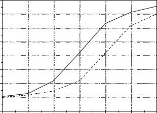
Figure 16.15 Comparison of average delay through the CPN with Bang-Bang control based on estimated delay.

by Equation (16.1). All the algorithms are allowed to use four items of information which are deposited in the nodes’ mailboxes:

(1)the length of the local queues in the node;

(2)recent values of the downstream delays experienced by packets which have previously gone through the output links and reached their destinations;

(3)the loss rate of packets which have passed through the same node and gone through the output links;

(4)estimates made by the most recent CPs which have used the output links headed for some destination d of its estimated delay Dd and loss Ld from this node to its destination.

The value Dd is updated by each successive CP passing through the node and whose destination is d. Samples of the simulation results are given in Figures 16.15–16.18.

16.6 GAME THEORY MODELS IN COGNITIVE RADIO NETWORKS

Game theory is a set of mathematical tools used to analyze interactive decision makers. We will show how these tools can be used in the analysis of cognitive networks [71–77]. The fundamental component of game theory is the concept of a game, formally expressed in normal form as [69, 70]:

G = N, A, {ui }