Advanced Wireless Networks - 4G Technologies

728 NETWORK INFORMATION THEORY

directivity antennas and antenna pointer tracking, the level of multiple access interference (MAI) and the required transmitted power are reduced. In order to exploit the available propagation diversity signals arriving from different directions (azimuth ψ , elevation ϕ) and delay τ are combined in a three-dimensional (ψ, ϕ, τ ) RAKE receiver. This is expected to significantly improve the system performance. In this section we present a systematic mathematical framework for capacity evaluation of such a CDMA network in the presence of implementation imperfections and a fading channel. The theory is general and some examples of a practical set of channel and system parameters are used as illustrations. As an example, it was shown that, in the case of voice applications and a two-dimensional (4 antennas×4 multipaths) RAKE receiver, up to 90 % of the system capacity can be lost due to the system imperfections. Further elaboration of these results, including extensive numerical analysis based on the offered analytical framework, would provide enough background for understanding of possible evolution of advanced W-CDMA and MC CDMA towards the fourth generation of mobile cellular communication networks.

The physical layer of the third generation of mobile communication system (3G) is based on wideband CDMA. The CDMA capacity analysis is covered in a number of papers and recently has become a subject in standard textbooks [2–8].

The effect of more sophisticated receiver structures (like multiuser detectors MUD or joint detectors) on CDMA or hybrid systems capacity has been examined in [9–13]. The results in H¨am¨al¨ainen et al. [9] show roughly twofold increase in capacity with MUD efficiency 65 % compared with conventional receivers. The effect of the fractional cell load on the coverage of the system is presented in [10]. The coverage of MUD-CDMA uplink was less affected by the variation in cell loading than in conventional systems. References [11] and [12] describe a CDMA system where joint data estimation is used with coherent receiver antenna diversity. This system can be used as hybrid multiple access scheme with TDMA and FDMA component. In Manji and Mandayam [13] significant capacity gains are reported when zero forcing multiuser detectors are used instead of conventional single-user receivers.

In most of the references it has been assumed that the service of interest is low rate speech. In next generation systems (4G), however, mixed services including high rate data have to be taken into account. This has been done in Huang and Bhargava [14], where the performance of integrated voice/data system is presented. It is also anticipated that 4G will be using adaptive antennas to further reduce the MAI. The effects of adaptive base station antenna arrays on CDMA capacity have been studied [6, 7]. The results show that significant capacity gains can be achieved with quite simple techniques.

One conventional way to improve cellular system capacity, used in 3G systems, is cell splitting, i.e. sub-dividing the coverage area of one base station to be covered by several base stations (smaller cells) [15]. Another simple and widely applied technique to reduce interference spatially in 3G is to divide cells into sectors, e.g. three 120◦ sectors. These sectors are covered by one or several directional antenna elements. The effects of sectorization to spectrum efficiency are studied in Chan [16]. The conclusion in Chan [16] is that sectorization reduces co-channel interference and improves the signal-to-noise ratio of the desired link at the given cluster size. However, at the same time the trunking efficiency is decreased [17]. Owing to the improved link quality, a tighter frequency reuse satisfies the performance criterion in comparison to the omnicellular case. Therefore, the net effect of sectorization is positive at least for large cells and high traffic densities.

By using M-element antenna arrays at the base station the spatial filtering effect can be further improved. The multiple beam adaptive array would not reduce the network trunking efficiency, unlike sectorization and cell splitting [18]. These adaptive or smart

antenna techniques can be divided into switched-beam, phased array and pure adaptive antenna systems. Advanced adaptive systems are also called spatial division multiple access (SDMA) systems. Advanced SDMA systems maximize the gain towards the desired mobile user and minimize the gain towards interfering signals in real time.

According to Winters [19], by applying a four-element adaptive array at the TDMA, uplink frequencies can be reused in every cell (three-sector system) and sevenfold capacity increase is achieved. Correspondingly, a four-beam antenna leads to reuse of three or four and doubled capacity at small angular spread.

Some practical examples of the impact of the use of advanced antenna techniques on the existing cellular standards are described in References [20, 21]. In Petrus et al. [20] the reference system is AMPS and in Mogensen et al. [21] it is GSM. The analysis in Kudoh and Matsumoto [22] uses ideal and flat-top beamformers. The main lobe of the ideal beamformer is flat and there are no sidelobes, whereas the flat-top beamformer has a fixed sidelobe level. The ideal beamformer can be seen as a realization of the underloaded system, i.e. there are less interferers than there are elements in the array. The overloaded case is better modeled by the flat-top beamformer because all interferers cannot be nulled and the sidelobe level is increased. Performance results show that reuse factor of one is not feasible in AMPS, but reuses four and three can be achieved with uniform linear arrays (ULA) with five and eight elements, respectively. Paper [21] concentrates on the design and performance of the frequency hopping GSM network using conventional beamforming. Most of the results are based on the simulated and measured data of eight-element ULA. The simulated C/I improvement follows closely the theoretical gain at low azimuth spreads. In urban macrocells the C/I gain is reduced from the theoretical value 9 dB down to approximately 5.5–7.5 dB. The designed direction of arrival (DoA) algorithm is shown to be very robust to co-channel interference. The potential capacity enhancement is reported to be threefold in a 1/3 reuse FH-GSM network for an array size of M = 4–6. A number of papers [23–30] present the analysis of capacity improvements using spatial filtering.

Solutions in 4G will go even beyond the above options and assume that both base station and the mobile unit are using beam forming and self-steering to continuously track transmitter–receiver direction (two side beam pointer tracking 2SBPT). Owing to user mobility and tracking imperfections there will be always tracking error that will result in lower received signal level, causing performance degradation. In this chapter we provide a general framework for performance analysis of a network using this technology. It is anticipated that this technology will be used in 4G systems.

19.1.1 4G cellular network system model

Although the general theory of MIMO system modeling is applicable for the system description, performance analysis will require more details and a slightly different approach will be used. This model will explicitly present signal parameters sensitive to implementation imperfections.

19.1.1.1 Transmitted signal

The complex envelope of the signal transmitted by user k {1, 2, . . . , K } in the nth symbol interval t [nT, (n + 1)T ] is

730 NETWORK INFORMATION THEORY

where Ak is the transmitted signal amplitude of user k, Tk (ψ, ϕ)is the transmitting antenna gain pattern as a function of azimuth ψ and elevation angle ϕ, τk is the signal delay, φk0 is the transmitted signal carrier phase, and Sk(n)(t) can be represented as

In this equation dik and dqk are two information bits in the I- and Q-channels, respectively,

and ci(nkm) and cqkm(n) are the mth chips of the kth user PN codes in the I- and Q-channel respectively. Equations (19.58) and (19.63) are general and different combinations of the

signal parameters over most of the signal formats of practical interest. In practical systems the codes will be a combination of a number of component codes [2].

19.1.1.2 Channel model

The channel impulse responses consist of discrete multipath components represented as

If antenna lobes are narrow we can use a discrete approximation of this functions in spatial domain too and implement 3D RAKE receive as follows:

where L is the overall number of spatial-delay multipath components of the channel. Each path is characterized by a specific angle of arrival (ψ, ϕ)and delay τ . Parameter h(kln) is the complex coefficient (gain) of the lth path of user k at symbol interval with index n, τkl(n) [0, Tm ) is the delay of the lth path component of user k in symbol interval n and δ(t) is the Dirac delta function. We assume that Tm is the delay spread of the channel. In what follows, indices n will be dropped whenever this does not produce any ambiguity. It is also assumed that Tm < T .

19.1.2 The received signal

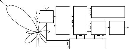
The base station receiver block diagram is shown in Figure 19.1 [31]. The overall received signal at the base station site during Nb symbol intervals can be represented as

Nb −1 K

Figure 19.1 Receiver block diagram.

where akl = Ak Tk (ψ, ϕ)Hkl(n)e j kl = Akl e j kl , Ak Tk (ψ, ϕ)Hkl(n) = Akl , kl = φ0 + φk0 −

φkl , φ0 is the frequency down-conversion phase error and z(t) is a complex zero mean additive white Gaussian noise process with two-sided power spectral density σ 2 and ω0 is the carrier frequency. In general, in the sequel we will refer to Akl as received signal amplitude. This amplitude will be further modified by the receiver antenna gain pattern. The complex matched filter of user k with receiver antenna pattern Rk (ψ, ϕ) will create two correlation functions for each path:

where ρx,y are cross-correlation functions between the corresponding code components x

and y. Each of these components is defined with three indices. Parameter = − ˜

εa,b a b

732 NETWORK INFORMATION THEORY

where a and b are defined with two indices each. In order to receive the incoming signal without any losses, the receiving antenna should be directing (pointing) the maximum of its radiation diagram towards the angle of arrival of the incoming signal. In this segment we will use the following terminology. The direction of the signal arrival is characterized by the pointer pa = (ψa, ϕa). In order to receive the maximum signal available, the receiver antenna pointer should be pr = (ψr, ϕr) = (ψa + π, ϕa + π ). Owing to mobility, the receiver will be tracking the incoming signal pointer and the pointer tracking error will be defined asp = pr − pa = (ψr − ψa, ϕr − ϕa) = ( ψ, ϕ). Owing to this error the amplitude of the received signal will be reduced by εp with respect to the maximum value. These issues will be elaborated later. When necessary, we should make a distinction between the amplitude seen by the receiver (asr) for a given pointer tracking error p and the maximum available amplitude (maa) obtained when p = 0. Let the vectors ( ) of MF output samples for the nth symbol interval be defined as

19.1.2.1 CDMA system capacity

The starting point in the evaluation of CDMA system capacity is the parameter Ym = Ebm /N0, the received signal energy per symbol per overall noise density in a given reference receiver with index m. For the purpose of this analysis we can represent this parameter in general case as

where Ioc, Ioic and Ioin are power densities of intracell-, intercelland overlay-type internetwork interference, respectively, and ηth is thermal noise power density. S is the overall received power of the useful signal and T = 1/Rb is the information bit interval. Contributions of Ioic and Ioin to N0 have been discussed in a number of papers [2]. In order to minimize repetition in our analysis, we will parameterize this contribution by introducing η0 = Ioic + Ioin + ηth and concentrate on the analysis of the intracell interference in the CDMA network based on advanced receivers using imperfect rake and MAI cancellation. A general block diagram of the receiver is shown in Figure 19.1. An extension of the analysis, to both intercell and internetwork interference, is straightforward.

19.1.3 Multipath channel: near–far effect and power control

We start with the rejection combiner, which will choose the first multipath signal component and reject (suppress) the others. In this case, Equation (19.9) for the I-channel becomes

where αx (z), (for x = iim1, iqm1, im1 and z = m1, k l ) is the power coefficient defined as αx (z) = Eε {|yx (z)|2}/S, S is normalized power level of the received signal and parameters yx (z) are in general defined by Equation (19.6).

K L

I (k l ) = αim1(k l )

k =1 l = 1(k =m)

l = 2(k = m)

is the equivalent MAI. Eε { } stands for averaging with respect to corresponding phases εa,b defined by Equation (19.7). Based on this, we have

where

ρi2m1(k l ) = ρi2k l ,im1 + ρqk2 l ,im1, ρ2 = Eρ ρi2k l ,im1 + ρqk2 l ,im1

and normalization A2k l ρ2/2 A2k l /2.

A similar equation can be obtained for the Q-channel too. It has been assumed that all ‘interference per path’ components are independent. In what follows we will simplify the notation by dropping all indices im1 so that αim1(k l ) αkl . With no power control (npc) αkl will depend only on the channel characteristics. In partial power control (ppc) only the first multipath component of the signal is measured and used in a power control (open or closed) loop. Full power control ( fpc) will normalize all components of the received signal and rake power control (rpc) will normalize only those components combined in the rake receiver. The (rpc) control seems to be more feasible because these components are already available. These concepts for ideal operation are defined by the following equations

where L0 is the number of fingers in the rake receiver. The contemporary theory in this field does not recognize these options which causes a lot of misunderstanding and misconceptions in the interpretation of the power control problem in the CDMA network. Although fpc is not practically feasible, the analysis including fpc should provide the reference results for the comparison with other, less efficient options. Another problem in the interpretation of the results in the analysis of the power control imperfections is caused by the assumption that all users in the network have the same problem with power control. Hence, the imperfect power control is characterized with the same variance of the power control error. This is more than pessimistic assumption and yet it has been used very often in analyses published so far. The above discussion is based on the signal amplitude seen by the receiver (asr). System losses due to difference between the asr and maa will be discussed in the next section. If we now introduce matrix αm with coefficients αkl , k, l except for αm1 = 0 and use notation 1 for vector of all ones, Equation (19.10) becomes

736 NETWORK INFORMATION THEORY

For a signal with the I- and Q-component the parameter cos εθr should be replaced by cos εθr cos εθr + mρ sin εθr , where m is the information in the interfering channel (I or Q), and ρ is the cross-correlation between the codes used in the I- and Q-channel. For small tracking errors this term can be replaced as cos εθr + mρ sin εθr ≈ 1 + mρε − ε2/2, where the notation is further simplified by dropping the subscript ( )θr . Similar expressions can be derived for the complex signal format. In the above discussion the signal amplitude seen by the receiver (asr) is used for Ar . In the presence of pointer estimation error this is related to the (maa) as Ar Ar − εp . So, to account for the losses due to εp, parameter αr in

ε¯ p and σp2 = E(ε2p ) are the mean and variance of the pointer tracking error. The power control will compensate for the pointer tracking losses by increasing the signal power by the amount equal to the losses. This means that the level of interference will be increased which can be taken into account in our model by modifying the parameters αkl as follows:

αkl αkl + 2¯εp √αkl − σpkl2

19.1.5 Interference canceler modeling: nonlinear multiuser detectors

For the system performance evaluation a model for the canceller efficiency is needed. Linear multiuser structure might not be of much interest in the next generation of the mobile communication systems where the use of long codes will be attractive. An alternative approach is nonlinear (multistage) multiuser detection, that would include channel estimation parameters too. This would be based on interference estimation and cancellation schemes (OKI standard-IS-665/ITU recommendation M.1073 or UMTS defined by ETSI)

In general if the estimates of Equation (19.8) are denoted yˆi and yˆq , then the residual interference after cancellation can be expressed as

where index ς k, l spans all combinations of k and l. By using Equation (19.22), each component αkl (1 − Ckl ) in Equation (19.16) can be obtained as a corresponding entry of Vec{| yς |2}.

To further elaborate these components we will use a simplified notation and analysis. After frequency downconversion and despreading, the signal from user k, received through path l at the receiver m, would have the form

correspond to yikl and yqkl . Parameter Amkl includes both amplitude and correlation function. In Equation (19.23) Amkl and εθ mkl are amplitude and phase estimation errors.