


Chapter 7
Quantum Harmonic Oscillator
A simple and interesting example of a dynamical system in quantum mechanics is the harmonic oscillator. This example is of importance for general theory, because it forms a corner-stone in the theory of radiation.
P.A. M. Dirac, The Principles of Quantum Mechanics
7.1Schr¨odinger Equation
In classical mechanics the state of a system consisting of N particles is specified by the position ~x and momentum p~ = m~v of each particle. The time evolution of this state is determined by solving Newton’s Second Law (or equivalently, say Hamilton’s equations). Thus, for example, a one particle system moving in three-dimensions (three degrees of freedom) determines a curve in 6-dimensional space: namely, (~x(t), p~(t)). For the familiar harmonic oscillator (mass-spring system) there is only one-degree of freedom (the movement of the mass is in one dimension only) and the position and momentum are given by the now familiar formulas1
x(t) |
= |
x0 cos(ω0t) + |
p0 |
sin(ω0t), |
(7.1) |
mω0 |
|||||
p(t) |
= |
p0 cos(ω0t) − mω0x0 sin(ω0t). |
(7.2) |
||
In quantum mechanics the notion of the state of the system is more abstract. The state is specified by a vector Ψ in some abstract vector space H. This vector space has an inner product (·, ·).2 Thus every state Ψ H satisfies
k Ψ k:= (Ψ, Ψ)1/2 < ∞. |
(7.3) |
1Actually, the second may look a little di erent from the earlier formulas. This is due to the fact that we are using momentum p instead of velocity v to describe the second coordinate of (x, p). Here p0 is the initial momentum and is related to the initial velocity by p0 = mv0.
2Such vector spaces are called Hilbert spaces.
97

98 |
CHAPTER 7. QUANTUM HARMONIC OSCILLATOR |
The importance of (7.3) is that in the Born interpretation |(Ψ, Φ)|2 is interpreted as a probability; and hence, must be finite (and less than or equal to one).3 In what is called the Schr¨odinger representation, one can describe the state Ψ as a function Ψ(x) where x is the position (of say the particle). Then |Ψ(x)|2 is the probability density of finding the particle in some small neighborhood of the point x. Integrating this over all possible positions must then give one.
The evolution of the state Ψ with time is determined by solving the Schr¨odinger equation:
i~ |
∂Ψ |
= HΨ. |
(7.4) |
∂t |
Here ~ is the Planck’s constant4 (divided by 2π) and H is the quantum mechanical Hamiltonian, a linear self-adjoint operator on the space H.5
7.2Harmonic Oscillator
7.2.1Harmonic Oscillator Equation
We illustrate the notions of quantum mechanics and its relationship to di erential equations in the context of the harmonic oscillator. The harmonic oscillator is one of the most important simple examples in quantum mechanics. In this case the vector space H is the space of square-integrable functions. This space consists of all (complex valued) functions ψ(x) such
that
Z ∞
|ψ(x)|2 dx < ∞.
−∞
This space is denoted by L2(R) and it comes equipped with an inner product
Z ∞
(ψ, ϕ) = ψ(x)ϕ¯(x) dx
−∞
where ϕ¯ is the complex conjugate of ϕ. (Note that in most physics books the complex conjugation is on the first slot.) The first observation, and an important one at that, is that the state space is infinite dimensional. For example, it can be proved that the infinite sequence of functions
xj e−x2 , j = 0, 1, 2 . . .
are linearly independent elements of L2(R). Thus in quantum mechanics one quickly goes beyond linear algebra which is traditionally restricted to finite-dimensional vector spaces.
3This assumes that states Ψ are normalized so that their “length” is one, i.e. k Ψ k= 1.
4In the cgs system, ~ = 1.05457 × 10⁻²⁷ erg-sec. A quantity that has the units of energy×time is called an action. In modern particle physics a unit system is adopted such that in these units ~ = 1. Max Planck received the Nobel prize in 1919 for “his discovery of energy quanta”.
5An operator H is self-adjoint if (Hψ, ψ) = (ψ, Hψ) for all ψ H. It is the generalization to Hilbert
spaces of the notion of a Hermitian matrix. There are some additional subtle questions regarding the domain of the operator H. In these notes we ignore such questions and assume H is well-defined on all states Ψ H.

7.2. HARMONIC OSCILLATOR |
99 |
The operator H which describes the harmonic oscillator can be defined once we give the quantization procedure—a heuristic that allows us to go from a classical Hamiltonian to a quantum Hamiltonian. As mentioned above, classically the state is given by the vector
(x, p) |
R2 |
. In quantum mechanics the |
position and momentum are replaced by operators |
||
|
2 |
2 |
(R) by |
||
xˆ and pˆ. For the vector space of states H = L |
(R), the position operator acts on L |
||||
multiplication,
(ˆxψ)(x) = xψ(x), ψ L2(R)
and the momentum operator pˆ acts by di erentiation followed by multiplication by the
constant −i~,
(pψˆ )(x) = −i~ ∂ψ∂x (x), ψ L2(R).
Since xˆ is multiplication by x we usually don’t distinguish between x and xˆ. From this we observe that in quantum mechanics the position operator and the momentum operator do not commute. To see this, let ψ L2(R), then
(ˆxpˆ − pˆxˆ) ψ(x) = −i~x |
∂ψ |
+ i~ |
∂ |
(xψ(x)) |
|
|
|||
∂x |
∂x |
=−i~x ∂ψ∂x + i~x ∂ψ∂x + i~ ψ(x)
=i~ ψ(x).
Introducing the commutator; namely, for any two operators A and B we define [A, B] =
AB − BA, the above can be written more compactly as6 |
|
[ˆx, pˆ] = i~ id |
(7.5) |
where by id we mean the identity operator. Equation (7.5) is at the heart of the famous
Heisenberg Uncertainty Relation.
With these rules we can now define the quantum harmonic oscillator Hamiltonian given the classical Hamiltonian (energy). Classically,7
E= KE + PE
= |
1 |
|
p2 + |
1 |
mω02 x2. |
|
2m |
2 |
|||||
|
|
|
||||
Replacing p → pˆ and x by multiplication by x we have
H = − ~2 d2 + 1 mω2x2 2m dx2 2 0
so that Schr¨odinger’s equation becomes
i~ |
∂Ψ |
= HΨ = − |
~2 d2Ψ |
+ |
1 |
mω02x2Ψ. |
(7.6) |
||
|
|
|
|
|
|||||
∂t |
2m dx2 |
2 |
|||||||
We first look for solutions in which the variables x and t separate
Ψ(x, t) = A(t)ψ(x).
6Just as in linear algebra, if A and B are two linear operators and it holds for all vectors ψ that Aψ = Bψ, then we can conclude that as operators A = B.
7Recall the potential energy for the harmonic oscillator is V (x) = 12 kx2 = 12 mω02 x2.

100 |
CHAPTER 7. |
QUANTUM HARMONIC OSCILLATOR |
|||||
Substituting this into (7.6) and dividing the result by A(t)ψ(x) we find |
|||||||
|
i~ |
1 |
|
dA |
= |
1 |
Hψ. |
|
|
|
|
||||
|
|
A dt |
ψ |
||||
Since the left hand side is only a function of t and the right hand side is only a function of x both sides must equal a common constant. Calling this constant E (observe this constant has the units of energy), we find
|
dA |
= |
− |
iE |
A, |
|
|
|
|
|
|
|
|||
|
dt |
~ |
|
||||
Hψ |
= |
Eψ. |
|
|
|||
The first equation has solution |
|
|
|
|
|
||
|
A(t) = e−iEt/~ |
|
|||||
so that |
|
|
|
|
|
||
Ψ(x, t) = e−iEt/~ ψ(x). |
(7.7) |
||||||
We now examine |
|
|
|
|
|
||
|
|
|
Hψ = Eψ |
|
(7.8) |
||
in detail. The first observation is that (7.8) is an eigenvalue problem in L2(R). Thus the eigenvalues of the operator H are interpreted as energies. It is convenient to introduce dimensionless variables to simplify notationally the di erential equation. Let
ξ = x r |
~ 0 |
, ε = |
~ω0 . |
|
|||
|
|
|
|
mω |
2E |
|
|
Performing this change of variables, the Schr¨odinger equation Hψ = Eψ becomes |
|
||||||
|
d2ψ |
|
|
||||
− |
|
+ (ξ2 − ε)ψ = 0. |
(7.9) |
||||
dξ2 |
|||||||
We want solutions to (7.9) that are square integrable. It is convenient to also perform a change in the dependent variable8
|
|
ψ(ξ) = e−ξ2 /2 v(ξ). |
|
||
Then a straightforward calculation shows that v must satisfy the equation |
|
||||
|
d2v |
− 2ξ |
dv |
|
|
|
|
|
+ (ε − 1)v = 0. |
(7.10) |
|
|
dξ2 |
dξ |
|||
Observe that (7.10) is not a constant coe cient di erential equation, so that the methods we have developed do not apply to this equation.
8This change of variables can be motivated by examining the asymptotic behavior of solutions near infinity and requiring the solutions be square integrable.

7.2. HARMONIC OSCILLATOR |
101 |
7.2.2 Hermite Polynomials |
|
To find solutions of (7.10) we look for solutions that are of the form9 |
|
∞ |
|
X |
|
v(ξ) = a0 + a1ξ + a2ξ2 + a3ξ3 + · · · = ak ξk . |
(7.11) |
k=0 |
|
The idea is to substitute this into (7.10) and to find conditions that the coe cients ak must satisfy. Since
|
|
|
|
|
|
|
dv |
|
|
∞ |
|
|
|
|
|
|
|
= a1 + 2a2 |
ξ + 3a3ξ2 + · · · = kak ξk−1 |
||
|
|
|
|
|
|
|
|
|||
|
|
|
|
|
|
|
dξ |
|||
|
|
|
|
|
|
|
|
|
|
k=1 |
and |
|
|
|
|
|
|
|
|
X |
|
|
d2v |
|
|
|
∞ |
|
∞ |
|||
|
|
|
|
|
|
|||||
|
|
|
= 2a2 + 6a3ξ + · · · = |
k(k |
− 1)ak ξk−2 = (k + 1)(k + 2)ak+2 ξk , |
|||||
|
|
|
dξ2 |
|||||||
|
|
|
|
|
|
|
|
k=2 |
k=0 |
|
we have |
|
|
X |
X |
||||||
|
|
|
|
|
||||||
|
d2v |
|
|
dv |
|
|
|
|
∞ |
|
|
− 2ξ |
+ (ε − 1)v = 2a2 + (ε − 1)a0 |
+ {(k + 2)(k + 1)ak+2 + (ε − 1 − 2k)ak} ξk . |
|||||||
|
dξ2 |
dξ |
||||||||
|
|
|
|
|
|
|
|
|
|
k=1 |
|
|
|
|
|
|
|
|
|
|
X |
For a power series to be identically zero, each of the co cients must be zero. Hence we obtain10
(k + 2)(k + 1)ak+2 + (ε − 1 − 2k) ak = 0, k = 0, 1, 2, . . . |
(7.12) |
Thus once a0 is specified, the coe cients a2, a4, a6, . . . are determined from the above recurrence relation. Similarly, once a1 is specified the coe cients a3, a5, a7, . . . are determined. The recurrence relation (7.12) can be rewritten as
|
ak+2 |
= |
2k − ε + 1 |
|
, k = 0, 1, 2, . . . |
(7.13) |
||
|
|
|
|
|||||
|
ak |
(k + 2)(k + 1) |
|
|||||
Our first observation from (7.13) is that |
|
= 0 |
|
|||||
|
|
|
k→∞ |
ak |
|
|||
|
|
|
lim |
|
ak+2 |
|
|
|
|
|
|
|
|
|
|
|
|
|
|
|
|
|
|
|
|
|
and so by the ratio test for power series, the radius of convergence of (7.11) is infinite. (This is good since we want our functions ψ to be defined for all ξ.)
Now comes a crucial point. We have shown for any choices of a0 and a1 and for any choice of the parameter (dimensionless energy) ε, that the function ψ(ξ) = e−ξ2/2v(ξ) solves the di erential equation (7.9) where v is given by (7.11) and the coe cients ak satisfy (7.13). However, a basic requirement of the quantum mechanical formalism is that ψ(ξ) is an element of the state space L2(R); namely, it is square integrable. Thus the question is whether e−ξ2/2v(ξ) is square integrable. We will show that we have square integrable functions for only certain values of the energy ε; namely, we will find the quantization of energy.
9This is called the power series method.
10Note that the k = 0 condition is a2 + (ε − 1)a0 = 0.

102 |
CHAPTER 7. |
QUANTUM HARMONIC OSCILLATOR |
|||
The ratio of the series coe cients, ak+1/ak, in the function |
|||||
|
eαz = ∞ ak zk |
= |
∞ |
αk zk |
|
|
X |
|
X |
|
|
|
k=0 |
|
k=0 |
k! |
|
|
|
|
|
||
is α/(k + 1) α/k as k → ∞. For the series (recall given a0 we can determine a2, a4, . . .)
∞∞
XX
v(ξ) = a2k ξ2k = bkzk, bk = a2k , z = ξ2,
k=0 k=0
the ratio of coe cients, bk+1/bk, is (we use (7.13) to get the second equality)
bk+1 |
= |
a2k+2 |
= |
4k − ε + 1 |
|
|
1 |
, k |
|
. |
bk |
|
|
k |
→ ∞ |
||||||
|
a2k |
(2k + 2)(2k + 1) |
|
|
||||||
This suggests in comparing the series for v with the series for eαz , and it can be proved,11
that
v(ξ) eξ2 , ξ → ∞.
Similar remarks hold for the series P∞ a2k+1ξ2k+1. This means our solution ψ(ξ) =
k=0
v(ξ)e−ξ2 /2 is not square integrable since it grows as eξ2 /2. Hence ψ is not a valid state in quantum mechanics. There is a way out of this: If the coe cients ak would vanish identically from some point on, then the solution v(ξ) will be a polynomial and thus ψ will be square integrable. From the recurrence relation (7.13) we see that this will happen if the numerator vanishes for some value of k. That is, if
ε = 2n + 1
for some nonnegative integer n, then an+2 = an+4 = · · · = 0. It is traditional to choose a normalization (which amounts to choices of a0 and a1) so that the coe cient of the highest power is 2n. With this normalization the polynomials are called Hermite polynomials and are denoted by Hn(ξ). The first few polynomials are12
H0(ξ) |
= |
1, |
|
H1(ξ) |
= |
2ξ, |
|
H2(ξ) = 4ξ2 − 2, |
|
||
H3(ξ) = 8ξ3 − 12ξ, |
|
||
H4(ξ) = 16ξ4 − 48ξ2 + 12, |
|
||
H5(ξ) |
= 32ξ5 − 160ξ3 + 120ξ, |
|
|
H6(ξ) |
= 64ξ4 − 480ξ4 + 720ξ2 − 120. |
|
|
Thus we have found solutions13 |
|
|
|
|
ψn(ξ) = NnHn(ξ)e−ξ2/2 |
(7.14) |
|
11This asymptotic analysis can be made rigorous using the theory of irregular singular points.
12One can compute a Hermite polynomial in MATHEMATICA by the command HermiteH[n,x] where n is a nonnegative integer.
13Here NN is an overall normalization constant which we choose below.

7.2. HARMONIC OSCILLATOR |
|
103 |
|
to (7.9); namely, |
|
|
|
Hψn = |
~ω0 |
(2n + 1)ψn, n = 0, 1, 2, . . . |
|
2 |
|||
|
|
We have solved an eigenvalue problem in the infinite dimensional space L2(R). It is convenient to choose the overall normalization constant Nn such that
k ψn k= 1, n = 0, 1, 2, . . .
That is, Nn is chosen so that
|
∞ |
|
Nn2 |
Z−∞ Hn(ξ)2e−ξ2 dξ = 1. |
(7.15) |
It can be shown that √
Nn = π n! 2n −1/2 .
7.2.3Quantization of Energy
The quantized energy levels are
1
En = 2 ~ω0 εn = ~ω0 (n + 1/2), n = 0, 1, 2, . . . .
That is to say, the energy of the quantum oscillator cannot have arbitrary real values (as in the case of the classical oscillator), but must be one of the discrete set of numbers
1 |
~ω0, |
3 |
~ω0, |
5 |
~ω0, . . . |
|
|
|
|||
2 |
2 |
2 |
The lowest energy, 12 ~ω0, is called the ground state energy and has associated wave function
ψ0(ξ) = 1 e−ξ2/2.
π1/4
Thus the ground state energy of the quantum harmonic oscillator is nonzero. In the classical harmonic oscillator, we can have p = x = 0 which corresponds to E = 0.
7.2.4Some properties of Hermite polynomials
Solution of Recurrence Relation
To obtain a more explicit formula for the Hermite polynomials we must solve the recurrence relation (7.13). The polynomials Hn(x) are normalized so that the coe cient of the highest power is 2n. This will determine a0 (when n is even) and a1 (when n is odd). We treat here the case of n even and leave the case of n odd to the reader. First
an |
= |
a2 |
|
a4 |
· · · |
an |
a0 |
a0 |
|
a2 |
an−2 |
104 |
CHAPTER 7. QUANTUM HARMONIC OSCILLATOR |
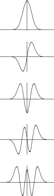
n=0 |
n=1 |
n=2 |
n=3 |
n=4 |
Figure 7.1: Harmonic Oscillator Wave Functions ψn(x) for n = 0, 1, 2, 3, 4.
7.2. HARMONIC OSCILLATOR |
|
|
|
|
|
|
|
|
|
|
105 |
||||||
The right hand side of this expression is determined from (7.13) and equals |
|||||||||||||||||
|
2(n) 2(n − 2) 2(n − 4) |
· · · |
2(2) |
|
|||||||||||||
|
|
|
|
|
|
|
|
|
|
|
|
|
|
|
|
|
|
|
1 |
· |
2 3 |
· |
4 |
5 |
· |
6 |
|
(n |
− |
1)n |
|||||
|
|
|
|
|
|||||||||||||
This can be rewritten as
2n/2n(n − 2)(n − 4) · · · 4 · 2
n!
This is the ratio an/a0. Requiring that an = 2n gives
a0 = 2n/2 (n − 1)(n − 3)(n − 5) · · · 5 · 3 · 1
We now determine am—the coe cient of xm— (when n is even we can take m even too).
Proceeding in a similar manner we write |
|
|
|
|
|||
|
am |
= |
a2 |
|
a4 |
· · · |
am |
|
a0 |
a0 |
|
a2 |
am−2 |
||
and again note the right hand side is determined from the recurrence relation (7.13); namely,
|
|
|
|
( |
1)m/2 |
2(n) |
|
2(n − 2) |
|
2(n − 4) |
|
2(n − m + 2) |
|
|||||||||||||
|
|
|
|
|
|
|
|
|||||||||||||||||||
|
|
|
|
− |
1 |
· |
2 3 |
· |
4 |
5 |
· |
6 |
· · · (m |
− |
1) |
· |
m |
|||||||||
|
|
|
|
|
|
|
|
|
|
|
|
|
|
|
|
|
|
|
|
|
|
|||||
Multiplying this by the value of a0 we get that am equals |
|
|
|
|
|
|||||||||||||||||||||
(−1) |
m/2 2(n+m)/2 |
|
|
|
|
|
|
|
|
|
|
|
|
|
|
|
|
|
|
|||||||
|
|
|
|
[n(n − 2)(n − 4) · · · (n − m + 2)] [(n − 1)(n − 3) · · · 5 · 3 · 1] |
||||||||||||||||||||||
|
|
m! |
|
|||||||||||||||||||||||
The product of the two quantities in square brackets can be rewritten as |
||||||||||||||||||||||||||
|
|
|
|
n! |
|
|
|
|
|
|
|
|
|
|
|
|
|
|
|
|
|
|
||||
|
|
|
|
|
|
(n − m − 1)(n |
− m − 3)(n − m − 5) |
· · ·5 · 3 · 1 |
||||||||||||||||||
|
|
|
(n |
− |
m)! |
|||||||||||||||||||||
|
|
|
|
|
|
|
|
|
|
|
|
|
|
|
|
|
|
|
|
|
|
|
|
|
|
|
Now let m → n − m (so am is the coe cient of xn−m ) to find that am equals
(−1)m/22n−m/2 n 1 · 3 · 5 · · ·(m − 1) m
|
n |
|
|
|
|
|
|
m → 2m |
|
|
|
|
|
||
where |
m |
is the binomial coe cient. Since m is even and runs over 0, 2, 4, . . . n, we can let |
|||||
|
|
to get the final formula14 |
|
|
|
|
|
|
|
[n/2] |
(−1)m |
|
|
||
|
|
Hn(x) = n! |
(2x)n−2m. |
(7.16) |
|||
|
|
X |
|
− |
2m)! |
|
|
|
|
m=0 m!(n |
|
|
|
||
This same formula holds for n odd if we interpret [n/2] = (n − 1)/2 when n is odd. From (7.16) we can immediately derive the di erentiation formula
dHn |
= 2n Hn−1(x). |
(7.17) |
|
dx
14We used the fact that
(2m − 1)!!/(2m)! = 1/(2M m!) where (2m − 1)!! = (2m − 1)(2m − 3) · · · 5 · 3 · 1.

106 CHAPTER 7. QUANTUM HARMONIC OSCILLATOR
Orthogonality Properties
The harmonic oscillator Hamiltonian H is self-adjoint with distinct eigenvalues. Just as we proved for matrices, it follows that that eigenfunctions ψn are orthogonal. The normalization constant Nn is chosen so that they are orthonormal. That is if ψn are defined by (7.14),
then |
∞ |
|
|
|
|
(ψn, ψm) = Nn2 |
Z−∞ Hn(x) Hm(x) e−x2 dx = δm,n |
(7.18) |
where Nn are defined in (7.15) and δm,n is the Kronecker delta function.15 The functions
ψn are called the harmonic oscillator wave functions.
From the orthogonality relations we can derive what is called the three-term recursion relation; namely, we claim that
Hn+1(x) − 2xHn(x) + 2nHn−1(x) = 0. |
(7.19) |
Since the highest power of Hn has coe cient 2n, we see that
Hn+1(x) − 2xHn(x)
must be a polynomial of degree less than or equal to n. Using (7.16) we can see that the highest power is the same as the highest power of 2n Hn−1(x). Thus the left hand side of (7.19) is a polynomial of degree less than or equal to n − 2. It can be written as the linear combination
c0 H0(x) + c1 H1(x) + · · · + cn−2 Hn−2(x).
We now multiply both sides of this resulting equation by Hk (x) e−x2 , 0 ≤ k ≤ n − 2, and integrate over all of R. Using the orthogonality relation one concludes that ck = 0.16
For applications to the harmonic oscillator, it is convenient to find what (7.16) and (7.19) imply for the oscillator wave functions ψn. It is an exercise to show that17
x ψn(x) =
dψn(x) = dx
r |
2 |
|
ψn−1(x) + r |
2 |
|
ψn+1(x) , |
(7.20) |
||
|
|
n |
|
|
n + 1 |
|
|
||
r |
|
|
|
ψn−1(x) − r |
|
|
|
ψn+1(x) . |
(7.21) |
|
|
|
|
2 |
|
||||
|
2 |
|
|
||||||
|
|
n |
|
|
n + 1 |
|
|
||
7.2.5Completeness of the harmonic oscillator wave functions {ψn}n≥0
In finite-dimensional vector spaces, we understand the notion of a basis. In particular, we’ve seen the importance of an orthonormal basis. In Hilbert spaces these concepts are
15δM,N equals 1 if m = n and 0 otherwise.
16Perhaps the only point that needs clarification is why
Z
2xHN (x)HK (x)e−X2 dx
R
is zero for 0 ≤ k ≤ n − 2. Since 2xHK (x) is a polynomial of degree k + 1 ≤ n − 1, it too can be expanded in terms of Hermite polynomials of degree less than or equal to n − 1; but these are all orthogonal to HN . Hence the expansion coe cients must be zero.
17These formulas are valid for n = 0 if we define ψ−1(x) = 0.