

6.8. VIBRATING MEMBRANE |
83 |
Writing (possible since the eigenvectors form a basis)
|
N |
|
|
|
|
X |
|
|
|
||
f = |
|
αnfN, |
|||
n=1 |
|
|
|
||
we conclude that |
|
|
|
|
|
N |
|
|
αn |
|
|
X |
|
|
|
|
|
|
ω2 |
− |
ω2 fN |
||
g = |
|
|
|||
n=1 |
n |
|
|
|
|
|
|
|
|
||
for ω2 6= ωn2 , n = 1, 2, . . . , N . The solution with initial values
u(0) = 0, u˙(0) = 0
is therefore of the form
N |
|
αn |
|
|
|
|
X |
|
|
|
|
X |
|
ω2 |
− |
ω2 fN |
+ |
|||
u(t) = cos ωt |
|
(an cos(ωnt) + bn sin(ωnt)) fN . |
||||
n=1 |
n |
|
|
|
|
n=1 |
|
|
|
|
|
||
Imposing the initial conditions (6.19) we obtain the two equations
n=1 ωn |
αn |
ω |
|
|
|
|
|
X |
|
− |
|
2 |
+ an fN |
= |
0, |
2 |
|
|
|||||
|
|
|
|
X |
|
|
|
|
|
|
|
|
ωnbnfN |
= |
0. |
n=1
From the fact that {fN}Nn=1 is a basis we conclude
an = − |
|
αn |
|
|
, bn |
= 0 for |
n = 1, 2, . . . , N. |
|
||||||||
ωn2 − ω2 |
|
|||||||||||||||
Thus the solution is |
|
|
|
|
|
|
|
|
|
|
|
|
|
|
|
|
N |
|
|
αn |
|
|
|
|
|
|
|
|
|
|
|
|
|
u(t) = |
|
|
|
|
(cos(ωt) − cos(ωnt)) fN |
|
|
|
|
|
||||||
ωn2 |
− |
ω2 |
|
|
|
|
|
|||||||||
n=1 |
|
|
|
|
|
|
|
|
|
|
|
|
|
|
|
|
X |
|
|
|
|
|
|
|
|
|
|
|
|
|
|
|
|
N |
|
2αn |
|
|
|
|
1 |
|
|
1 |
|
|
|
|
||
= |
|
|
sin |
(ωn + ω)t |
sin |
(ωn |
|
ω)t |
fN . |
|||||||
2 |
|
ω |
2 |
2 |
|
− |
||||||||||
n=1 |
ωn |
− |
|
|
|
|
2 |
|
|
|
||||||
X |
|
|
|
|
|
|
|
|
|
|
|
|
|
|
|
|
(6.19)
(6.20)
(6.21)
(6.22)
(6.23)
We observe that there is a beat whenever the driving frequency ω is close to a normal mode of oscillation ωn. Compare this discussion with that of Boyce & DiPrima [4].
6.8Vibrating Membrane
6.8.1Helmholtz Equation
In the previous section we discussed the vibrating string. Recall that we have a string of unstretched length L that is tied down at ends 0 and L. If u = u(x; t) denotes the vertical

84 |
CHAPTER 6. WEIGHTED STRING |
displacement of the string at position x, 0 ≤ x ≤ L, at time t, then we showed that for small displacements u satisfies the one-dimensional wave equation
∂2u 1 ∂2u ∂x2 − v2 ∂t2 = 0
where v2 = T /µ, T equals the tension in string and µ is the density of the string. We solved this equation subject to the boundary conditions u(0, t) = u(L, t) = 0 for all t and with initial conditions u(x, 0) = f (x) and ∂u∂t (x, 0) = g(x) where f and g are given.
Now we imagine a uniform, flexible membrane, of mass ρ per unit area, stretched under a uniform tension T per unit length over a region Ω in the plane whose boundary ∂Ω is a smooth curve (with a possible exception of a finite number of corners).
We now let U = U (x, y; t) denote the vertical displacement of the membrane at position (x, y) Ω at time t from its equilibrium position. We again assume that the membrane is tied down at the boundary; that is1
U (x, y; t) = 0 for (x, y) ∂Ω.
The motion of U = U (x, y; t) is governed by the two-dimensional wave equation:
|
|
∂2U ∂2U |
1 |
|
∂2U |
|
(6.24) |
||||
|
|
|
|
|
|
|
|
|
|
|
|
|
|
∂x2 + ∂y2 − v2 |
|
∂t2 |
= 0 for (x, y) Ω |
||||||
|
|
|
|
||||||||
where v2 = T /ρ. One recognizes ∂2 U2 |
+ |
∂2U2 |
as the two-dimensional Laplacian. So if we |
||||||||
|
|
|
|
∂x |
|
|
∂y |
|
|
||
introduce
∂∂
=∂x2 + ∂y2
the wave equation takes the form
1 ∂2U
U − v2 ∂t2 = 0.
We proceed as before an look for solutions of (6.24) in which the variables separate
U (x, y; t) = u(x, y)T (t).
Substituting this into (6.24), dividing by uT gives
1 |
|
1 1 d2T |
|||||
|
u = |
|
|
|
|
|
. |
u |
v2 |
T |
dt2 |
||||
The right-hand side depends only upon t where as the left-hand side depends only upon x, y. Thus for the two sides to be equal they must equal the same constant. Call this constant −k2. Thus we have the two equations
1In one dimension Ω = (0, L) and the boundary of Ω consists of the two points 0 and L.
6.8. VIBRATING MEMBRANE |
|
|
85 |
||
|
d2T |
+ ω2T |
= |
0 where ω = kv, |
|
|
|
|
|||
|
dt2 |
|
|
|
|
|
u + k2u |
= |
0. |
(6.25) |
|
The di erential equation for T has our well-known solutions
eiωt and e−iωt.
The second equation (6.25), called the Helmholtz equation, is a partial di erential equation for u = u(x, y). We wish to solve this subject to the boundary condition
u(x, y) = 0 for (x, y) ∂Ω.
6.8.2Rectangular Membrane
Consider the rectangular domain
Ω = {(x, y) : 0 < x < a, 0 < y < b} |
(6.26) |
For this rectangular domain the Helmholtz equation can be solved by the method of separation of variables. If one assumes a solution of the form (variables x and y separate)
u(x, y) = X(x)Y (y)
then the problem is reduced to two one-dimensional problems. It is an exercise to show that the allowed frequencies are
ωm,n = πv |
a |
|
2 |
+ |
b |
2 |
|
1/2 |
(6.27) |
|||
, m, n = 1, 2, 3, . . . |
||||||||||||
|
|
m |
|
|
|
n |
|
|
|
|
||
6.8.3 Circular Membrane: The Drum
We now consider the circular domain
Ω = (x, y) : x2 + y2 < a2
so the boundary of Ω is the circle ∂Ω : x2 + y2 = a2. Even though the variables separate in the Cartesian coordinates x and y, this is of no use since the boundary is circular and we would not be able to apply the BC u = 0 on the circular boundary ∂Ω. Since the domain is circular it is natural to introduce polar coordinates
x = r cos θ, y = r sin θ.
It is an exercise in the chain rule to show that in polar coordinates the 2D Laplacian is
u = |
∂2u |
1 |
|
∂u |
|
1 ∂2u |
|
|||
|
+ |
|
|
|
+ |
|
|
|
; |
|
∂r2 |
r |
∂r |
r2 |
∂θ2 |
||||||
and hence, the Helmholtz equation in polar coodinates is
∂2u |
+ |
1 |
|
∂u |
1 |
|
∂2u |
+ k2u = 0. |
(6.28) |
|
|
|
|
|
+ |
|
|
|
|||
∂r2 |
|
|
r2 |
|
∂θ2 |
|||||
|
r ∂r |
|
|
|
||||||
We write u = u(r, θ).2
2Possible point of confusion: We wrote u = u(x, y) so really our new function of r and θ is u(r cos θ, r sin θ). Technically we should give this function of r and θ a new name but that would be rather pedantic.
86 |
CHAPTER 6. WEIGHTED STRING |
Separation of Variables
We now show that the variables separate. So we look for a solution of the form
u(r, θ) = R(r)Θ(θ).
Substituting this into (6.28), multiplying by r2/RΘ we have
r2 d2R |
+ |
r dR |
+ k2r2 |
= − |
1 d2Θ |
||||||
|
|
|
|
|
|
|
|
|
|||
R |
dr2 |
R |
dr |
Θ dθ2 |
|||||||
By the now familiar argument we see that each of the above sides must equal a constant, call it m2, to obtain the two di erential equations
|
|
|
|
|
|
d2Θ |
+ m2Θ |
= |
0 |
(6.29) |
||
|
|
|
|
|
|
dθ2 |
||||||
|
|
|
|
|
|
|
|
|
|
|
|
|
d2R |
1 |
|
dR |
+ (k2 − |
m2 |
|
|
|
||||
|
+ |
|
|
|
|
)R |
= |
0 |
(6.30) |
|||
dr2 |
r |
|
dr |
r2 |
||||||||
Two linearly independent solutions to (6.29) are
eimθ and e−imθ
The point with polar coordinates (r, θ) is the same point as the one with polar coordinates (r, θ + 2π). Thus our solution u(r, θ) and u(r, θ + 2π) must be the same solution. This
requires
eimθ+im2π = eimθ
or e2πim = 1. That is, m must be an integer. If m = 0 the general solution to (6.29) is c1 + c2θ. But the θ → θ + 2π argument requires we take c2 = 0. Thus the general solution to (6.29) is
am cos(mθ) + bm sin(mθ), m = 0, 1, 2, . . .
We now return to (6.30), called the Bessel equation, which is a second order linear di erential equation. General theory tells us there are two linearly independent solutions. Tradition has it we single out two solutions. One solution, called Jm(kr), is finite as r → 0 and the other solution, called Ym(kr) goes to infinity as r → 0. Both of these functions are called Bessel functions. It can be shown that the Bessel function Jm(z) is given by the series expansion
Jm(z) = |
z |
|
m ∞ |
1 |
|
|
z |
|
2j |
2 |
j=0(−1)j j!(m + j)! |
2 |
(6.31) |
||||||
|
|
|
X |
|
|
|
|
|
|
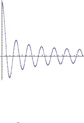
A plot of the Bessel function J0(x) for 0 ≤ x ≤ 40 is given in Figure 6.4. In Mathematica, Bessel functions Jm(z) are called by the command BesselJ[m,z]. Since u(r, θ) is welldefined at r = 0 (center of the drum), this requires we only use the Jm solutions. Thus we have shown that
Jm(kr) (am cos(mθ) + bm sin(mθ)) , m = 0, 1, 2, . . .
are solutions to (6.28). We now require that these solutions vanish on ∂Ω. That is, when r = a and for all θ we require the above solution to vanish. This will happen if
Jm(ka) = 0.
6.8. VIBRATING MEMBRANE |
87 |
Bessel Function J0
1.0 |
|
|
|
0.8 |
|
|
|
0.6 |
|
|
|
0.4 |
|
|
|
0.2 |
|
|
|
10 |
20 |
30 |
40 |
-0.2 |
|
|
|
-0.4 |
|
|
|
Figure 6.4: The Bessel function J0(x). First zero occurs at approximately 2.4048, the second zero at 5.5201, the third zero at 8.6537, . . . .
That is we have to be at a zero of the Bessel function Jm. It is known that Jm has an infinite number of real zeros, call them jm,n, n = 1, 2, . . .. Thus the frequencies that the drum can oscillate at are
where jm,n is the nth zero of the Bessel function Jm(z). These zeros can be found in Mathematica using the command BesselJZero[m,n].
6.8.4Comments on Separation of Variables
For general domains Ω one cannot solve the Helmholtz equation (6.25) by the method of separation of variables. In general if one makes the transformations x = f (ξ, η) and y = g(ξ, η) then one would want the curves of constant ξ (or constant η) to describe the boundary ∂Ω and for Helmholtz’s equation to separate variables in the new variables ξ and η. In general there are no such coordinates. For an elliptical membrane the Helmholtz equation does separate in what are called elliptic coordinates
x = |
c |
cosh µ cos θ, |
y = |
c |
sinh µ sin θ |
|
2 |
2 |
|||||
|
|
|
|
where c R+, 0 < µ < ∞ and 0 ≤ θ ≤ 2π. The curves µ = constant and θ = constant are confocal ellipses and hyperbolas, respectively. Qualitative new phenomena arise for elliptical (and more generally convex) membranes: the existence of whispering gallery modes and bouncing ball modes. In the whispering gallery mode the eigenfunction is essentially nonzero