

Lectures on Di erential Equations1
Craig A. Tracy2
Department of Mathematics
University of California
Davis, CA 95616
March 2011
1 c Craig A. Tracy, 2000, 2005, 2011 Davis, CA 95616 2email: tracy@math.ucdavis.edu
2
Contents
1 Pendulum and MatLab |
1 |
1.1 Di erential Equations . . . . . . . . . . . . . . . . . . . . . . . . . . . . . . . |
1 |
1.2Introduction to MatLab . . . . . . . . . . . . . . . . . . . . . . . . . . . . . . 4
1.3 Exercises . . . . . . . . . . . . . . . . . . . . . . . . . . . . . . . . . . . . . . |
5 |
2 First Order Equations |
9 |
2.1Linear First Order Equations . . . . . . . . . . . . . . . . . . . . . . . . . . . 9
2.2Separation of Variables Applied to Mechanics . . . . . . . . . . . . . . . . . . 14
2.3 Exercises . . . . . . . . . . . . . . . . . . . . . . . . . . . . . . . . . . . . . . |
23 |
3 Second Order Linear Equations |
31 |
3.1Theory of Second Order Equations . . . . . . . . . . . . . . . . . . . . . . . . 31
3.2Reduction of Order . . . . . . . . . . . . . . . . . . . . . . . . . . . . . . . . . 35
3.3Constant Coe cients . . . . . . . . . . . . . . . . . . . . . . . . . . . . . . . . 35
3.4 |
Forced Oscillations of the Mass-Spring System . . . . . . . . . . . . . . . . . |
40 |
3.5 |
Exercises . . . . . . . . . . . . . . . . . . . . . . . . . . . . . . . . . . . . . . |
44 |
4 Di erence Equations |
47 |
|
4.1Introduction . . . . . . . . . . . . . . . . . . . . . . . . . . . . . . . . . . . . . 47
4.2Constant Coe cient Di erence Equations . . . . . . . . . . . . . . . . . . . . 48
4.3Inhomogeneous Di erence Equations . . . . . . . . . . . . . . . . . . . . . . . 50
4.4 Exercises . . . . . . . . . . . . . . . . . . . . . . . . . . . . . . . . . . . . . . 50
i
ii |
|
|
CONTENTS |
|
5 |
Matrix Di erential Equations |
|
53 |
|
|
5.1 |
The Matrix Exponential . . . . . . . . . . . . . . . . . . . . . . . |
. . . . . . . |
53 |
|
5.2 |
Application of Matrix Exponential to DEs . . . . . . . . . . . . . |
. . . . . . . |
56 |
|
5.3 |
Relation to Earlier Methods of Solving Constant Coe cient DEs |
. . . . . . . |
59 |
|
5.4 |
Inhomogenous Matrix Equations . . . . . . . . . . . . . . . . . . |
. . . . . . . |
60 |
|
5.5 |
Exercises . . . . . . . . . . . . . . . . . . . . . . . . . . . . . . . |
. . . . . . . |
61 |
6 |
Weighted String |
|
67 |
|
6.1Derivation of Di erential Equations . . . . . . . . . . . . . . . . . . . . . . . . 67
6.2Reduction to an Eigenvalue Problem . . . . . . . . . . . . . . . . . . . . . . . 70
6.3Computation of the Eigenvalues . . . . . . . . . . . . . . . . . . . . . . . . . . 70
6.4The Eigenvectors . . . . . . . . . . . . . . . . . . . . . . . . . . . . . . . . . . 72
6.5 Determination of constants . . . . . . . . . . . . . . . . . . . . . . . . . . . . 75
6.6Continuum Limit: The Wave Equation . . . . . . . . . . . . . . . . . . . . . . 79
6.7Inhomogeneous Problem . . . . . . . . . . . . . . . . . . . . . . . . . . . . . . 82
6.8Vibrating Membrane . . . . . . . . . . . . . . . . . . . . . . . . . . . . . . . . 83
6.9 |
Exercises . . . . . . . . . . . . . . . . . . . . . . . . . . . . . . . . . . . . . . |
88 |
7 Quantum Harmonic Oscillator |
97 |
|
7.1 |
Schr¨odinger Equation . . . . . . . . . . . . . . . . . . . . . . . . . . . . . . . |
97 |
7.2 |
Harmonic Oscillator . . . . . . . . . . . . . . . . . . . . . . . . . . . . . . . . |
98 |
7.3Some properties of the harmonic oscillator . . . . . . . . . . . . . . . . . . . . 107
7.4 |
The Heisenberg Uncertainty Principle |
. . . . . . . . . . . . . . . . . . . . . . 111 |
|
7.5 |
Exercises . . . . . . . . . . . . . . . |
. . . . . . . . . . . . . . . . . . . . . . . |
113 |
8 Laplace Transform |
|
115 |
|
8.1 |
Matrix version . . . . . . . . . . . . |
. . . . . . . . . . . . . . . . . . . . . . . |
115 |
8.2Structure of (sIn − A)−1 . . . . . . . . . . . . . . . . . . . . . . . . . . . . . . 119
8.3 Exercises . . . . . . . . . . . . . . . . . . . . . . . . . . . . . . . . . . . . . . 120
CONTENTS |
iii |
Preface
These lecture notes are meant for a one-quarter course in di erential equations. Typically I do not cover the last section on Laplace transforms but it is included as a future reference for the engineers who will need this material.
I wish to thank Eunghyun (Hyun) Lee for his help with these notes during the 2008–09 academic year.
As a preface to the study of di erential equations one can do no better than to quote V. I. Arnold, Geometrical Methods in the Theory of Ordinary Di erential Equations:
Newton’s fundamental discovery, the one which he considered necessary to keep secret and published only in the form of an anagram, consists of the following:
Data aequatione quotcunque fluentes quantitae involvente fluxions invenire et vice versa. In contemporary mathematical language, this means: “It is useful to solve di erential equations”.
Craig Tracy, Sonoma, California
iv |
CONTENTS |
|
Notation |
Symbol |
Definition of Symbol |
R |
field of real numbers |
Rn |
the n-dimensional vector space with each component a real number |
C |
field of complex numbers |
x˙ |
the derivative dx/dt, t is interpreted as time |
x¨ |
the second derivative d2x/dt2, t is interpreted as time |
:= |
equals by definition |
Ψ = Ψ(x, t) |
wave function in quantum mechanics |
ODE |
ordinary di erential equation |
PDE |
partial di erential equation |
KE |
kinetic energy |
PE |
potential energy |
det |
determinant |
δij |
the Kronecker delta, equal to 1 if i = j and 0 otherwise |
Ln |
the Laplace transform operator |
k |
The binomial coe cient n choose k. |
M |
is a registered trademark of Maplesoft. |
APLE |
|
MATHEMATICA |
is a registered trademark of Wolfram Research. |
MATLAB |
is a registered trademark of the MathWorks, Inc. |
Chapter 1
Mathematical Pendulum
Newton’s principle of determinacy
The initial state of a mechanical system (the totality of positions and velocities of its points at some moment of time) uniquely determines all of its motion.
It is hard to doubt this fact, since we learn it very early. One can imagine a world in which to determine the future of a system one must also know the acceleration at the initial moment, but experience shows us that our world is not like this.
V.I. Arnold, Mathematical Methods of Classical Mechanics[1]
1.1Derivation of the Di erential Equations
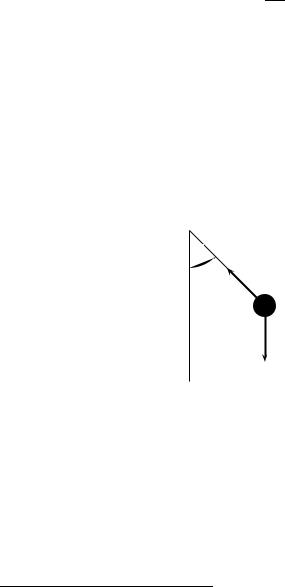
Many interesting ordinary di erential equations (ODEs) arise from applications. One reason for understanding these applications in a mathematics class is that you can combine your physical intuition with your mathematical intuition in the same problem. Usually the result is an improvement of both. One such application is the motion of pendulum, i.e. a ball of mass m suspended from an ideal rigid rod that is fixed at one end. The problem is to describe the motion of the mass point in a constant gravitational field. Since this is a mathematics class we will not normally be interested in deriving the ODE from physical principles; rather, we will simply write down various di erential equations and claim that they are “interesting.” However, to give you the flavor of such derivations (which you will see repeatedly in your science and engineering courses), we will derive from Newton’s equations the di erential equation that describes the time evolution of the angle of deflection of the pendulum.
Let
ℓ= length of the rod measured, say, in meters,
m= mass of the ball measured, say, in kilograms,
g= acceleration due to gravity = 9.8070 m/s2.
The motion of the pendulum is confined to a plane (this is an assumption on how the rod is attached to the pivot point), which we take to be the xy-plane. We treat the ball as a
1
2 |
CHAPTER 1. PENDULUM AND MATLAB |
“mass point” and observe there are two forces acting on this ball: the force due to gravity,
~
mg, which acts vertically downward and the tension T in the rod (acting in the direction indicated in figure). Newton’s equations for the motion of a point ~x in a plane are vector equations1
~
F = m~a
~
where F is the sum of the forces acting on the the point and ~a is the acceleration of the point, i.e.
d2~x ~a = dt2 .
In x and y coordinates Newton’s equations become two equations
Fx = m |
d2x |
, Fy = m |
d2y |
, |
dt2 |
dt2 |
~
where Fx and Fy are the x and y components, respectively, of the force F . From the figure
~
(note definition of the angle θ) we see, upon resolving T into its x and y components, that
Fx = −T sin θ, Fy = T cos θ − mg.
~
(T is the magnitude of the vector T .)
θℓ
T
mass m
mg
Substituting these expressions for the forces into Newton’s equations, we obtain the di erential equations
− T sin θ |
|
|
d2x |
|
||
= |
m |
|
|
, |
(1.1) |
|
dt2 |
||||||
T cos θ − mg |
= |
m |
d2y |
|
||
|
. |
(1.2) |
||||
dt2 |
||||||
From the figure we see that |
|
|
|
|
|
|
x = ℓ sin θ, y = ℓ − ℓ cos θ. |
(1.3) |
|||||
1In your applied courses vectors are usually denoted with arrows above them. We adopt this notation when discussing certain applications; but in later chapters we will drop the arrows and state where the quantity lives, e.g. x R2.

1.1. DIFFERENTIAL EQUATIONS |
3 |
(The origin of the xy-plane is chosen so that at x = y = 0, the pendulum is at the bottom.) Di erentiating2 (1.3) with respect to t, and then again, gives
x˙ |
= |
˙ |
|
|
ℓ cos θ θ, |
|
|
||
x¨ |
= |
¨ |
˙ 2 |
(1.4) |
ℓ cos θ θ − ℓ sin θ (θ) , |
||||
y˙ |
= |
˙ |
|
|
ℓ sin θ θ, |
|
|
||
y¨ |
= |
¨ |
˙ 2 |
(1.5) |
ℓ sin θ θ + ℓ cos θ (θ) . |
||||
Substitute (1.4) in (1.1) and (1.5) in (1.2) to obtain |
|
|
||
− T sin θ |
¨ |
˙ 2 |
(1.6) |
|
= mℓ cos θ θ |
− mℓ sin θ (θ) , |
|||
T cos θ − mg |
¨ |
˙ 2 |
(1.7) |
|
= mℓ sin θ θ + mℓ cos θ (θ) . |
||||
Now multiply (1.6) by cos θ, (1.7) by sin θ, and add the two resulting equations to obtain
|
|
|
¨ |
|
|
−mg sin θ = mℓθ, |
|
||
or |
|
|
|
|
|
|
|
|
|
|
¨ |
g |
|
|
|
θ + |
ℓ |
sin θ = 0. |
(1.8) |
|
|
|
||
|
|
|
|
|
|
|
|
|
|
Remarks
•The ODE (1.8) is called a second-order equation because the highest derivative appearing in the equation is a second derivative.
•The ODE is nonlinear because of the term sin θ (this is not a linear function of the unknown quantity θ).
•A solution to this ODE is a function θ = θ(t) such that when it is substituted into the ODE, the ODE is satisfied for all t.
•Observe that the mass m dropped out of the final equation. This says the motion will be independent of the mass of the ball.
• |
~ |
The derivation was constructed so that the tension, T , was eliminated from the equa- |
|
|
tions. We could do this because we started with two unknowns, T and θ, and two |
|
equations. We manipulated the equations so that in the end we had one equation for |
|
the unknown θ = θ(t). |
•We have not discussed how the pendulum is initially started. This is very important and such conditions are called the initial conditions.
We will return to this ODE later in the course. At this point we note that if we were interested in only small deflections from the origin (this means we would have to start out near the origin), there is an obvious approximation to make. Recall from calculus the Taylor
expansion of sin θ
sin θ = θ − θ3 + θ5 + · · · . 3! 5!
For small θ this leads to the approximation sin θ ≈ θ . Using this small deflection approximation in (1.8) leads to the ODE
2We use the dot notation for time derivatives, e.g. x˙ = dx/dt, x¨ = d2x/dt2.

4 |
CHAPTER 1. PENDULUM AND MATLAB |
¨ |
g |
|
(1.9) |
θ + |
ℓ |
θ = 0. |
|
|
|
|
|
|
|
|
|
We will see that (1.9) is mathematically simpler than (1.8). The reason for this is that (1.9) is a linear ODE. It is linear because the unknown quantity, θ, and its derivatives appear only to the first or zeroth power.
1.2Introduction to MatLab
In this class we will use the computer software package MATLAB to do routine calculations. It will take the drudgery out of linear algebra! Engineers will find that MATLAB is used extensively in their upper division classes so learning it now is a good investment. What is MATLAB ? “MATLAB is a powerful computing system for handling the calculations involved in scientific and engineering problems.”3 MATLAB can be used either interactively or as a programming language. For most applications in Math 22B it su ces to use MATLAB interactively. Typing matlab at the command level is the command for most systems to start MATLAB . Once it loads you are presented with a prompt sign >>. For example if I enter
>> 2+22
and then press the enter key it responds with
ans=24
Multiplication is denoted by * and division by / . Thus, for example, to compute
(139.8)(123.5 − 44.5)
125
we enter
>> 139.8*(123.5-44.5)/125
gives
ans=88.3536
MATLAB also has a Symbolic Math Toolbox which is quite useful for routine calculus computations. For example, suppose you forgot the Taylor expansion of sin x that was used in the notes just before (1.9). To use the Symbolic Math Toolbox you have to tell MATLAB that x is a symbol (and not assigned a numerical value). Thus in MATLAB
3Brian D. Hahn, Essential MATLAB for Scientists and Engineers.
1.3. EXERCISES |
5 |
>>syms x
>>taylor(sin(x))
gives
ans = x -1/6*x^3+1/120*x^5
Now why did taylor expand about the point x = 0 and keep only through x5? By default the Taylor series about 0 up to terms of order 5 is produced. To learn more about taylor enter
>> help taylor
from which we learn if we had wanted terms up to order 10 we would have entered
>> taylor(sin(x),10)
If we want the Taylor expansion of sin x about the point x = π up to order 8 we enter
>> taylor(sin(x),8,pi)
A good reference for MATLAB is MatLab Guide by Desmond Higham and Nicholas Higham.
There are alternatives to the software package MATLAB. Two widely used packages are MATHEMATICA and MAPLE. In MATHEMATICA to find the Taylor series of sin x about the point x = 0 to fifth order you would type
Series[Sin[x],x,0,5]
1.3Exercises
#1. MatLab Exercises
1.Use MATLAB to get an estimate (in scientific notation) of 9999. Now use
>>help format
to learn how to get more decimal places. (All MATLAB computations are done to a relative precision of about 16 decimal places. MATLAB defaults to printing out the first 5 digits.) Thus entering
>> format long e
on a command line and then re-entering the above computation will give the 16 digit answer.

6 |
|
|
|
|
CHAPTER 1. PENDULUM AND MATLAB |
|
|
|
|
||
2. Use MATLAB to compute |
|
sin(π/7). (Note that MATLAB has the special symbol pi; |
|||
that is |
pi |
|
. . to 16 digits accuracy.) |
||
|
≈ π = 3.14159 . p |
||||
3. Use MATLAB to find the determinant, eigenvalues and eigenvectors of the 4 ×4 matrix
A = |
√2 |
1 |
0 |
−2 |
|
|||
|
|
1 |
−1 |
2 |
0 |
|
||
|
|
|
|
|
√ |
|
|
|
|
1 |
2 |
|
0 |
||||
|
2 |
|
||||||
|
|
0 |
1 |
|
|
−1 |
|
|
|
|
|
|
|
|
|
|
|
Hint: In MATLAB you enter the matrix A by
>> A=[1 -1 2 0; sqrt(2) 1 0 -2;0 1 sqrt(2) -1; 1 2 2 0]
To find the determinant
>> det(A)
and to find the eigenvalues
>> eig(A)
If you also want the eigenvectors you enter
>> [V,D]=eig(A)
In this case the columns of V are the eigenvectors of A and the diagonal elements of D are the corresponding eigenvalues. Try this now to find the eigenvectors. For the determinant you should get the result 16.9706. One may also calculate the determinant symbolically. First we tell MATLAB that A is to be treated as a symbol (we are assuming you have already entered A as above):
>> A=sym(A)
and then re-enter the command for the determinant
det(A)
and this time MATLAB returns
ans = 12*2^(1/2)
√
that is, 12 2 which is approximately equal to 16.9706.
4. Use MATLAB to plot sin θ and compare this with the approximation sin θ ≈ θ. For 0 ≤ θ ≤ π/2, plot both on the same graph. Here is the MATLAB code that puts both graphs in the same plot:
>> x=0:.01:pi/2; plot(x,sin(x),x,x)
1.3. EXERCISES |
7 |
#2. Inverted Pendulum
This exercise derives the small angle approximation to (1.8) when the pendulum is nearly inverted, i.e. θ ≈ π. Introduce
φ = θ − π
and derive a small φ-angle approximation to (1.8). How does the result di er from (1.9)?
8 |
CHAPTER 1. PENDULUM AND MATLAB |