

Chapter 6
Weighted String
Because linear equations are easy to solve and study, the theory of linear oscillations is the most highly developed area of mechanics. In many nonlinear problems, linearization produces a satisfactory approximate solution. Even when this is not the case, the study of the linear part of a problem is often a first step, to be followed by the study of the relation between motions in a nonlinear system and its linear model.
V.I. Arnold, Mathematical Methods of Classical Mechanics [1]
6.1Derivation of Di erential Equations
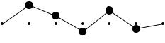
The weighted string is a system in which the mass is concentrated in a set of equally spaced mass points, N in number with spacing d, imagined to be held together by massless springs of equal tension T . We further assume that the construction is such that the mass points move only in the vertical direction (y direction) and there is a constraining force to keep the mass points from moving in the horizontal direction (x direction). We call it a “string” since these mass points give a discrete string—the tension in the string is represented by the springs. The figure below illustrates the weighted string for N = 5.
0 |
1d |
2d |
3d |
4d |
5d |
6d |
The string is “tied down” at the endpoints 0 and (N + 1)d. The horizontal coordinates of the mass points will be at x = d, 2d, . . . , N d. We let uj denote the vertical displacement of the jth mass point and Fj the transverse force on the jth particle. To summarize the
67
68 |
CHAPTER 6. WEIGHTED STRING |
variables introduced so far:
m |
= |
mass of particle, |
N |
= |
total number of particles, |
T |
= |
tension of spring, |
d |
= horizontal distance between two particles, |
|
uj |
= |
vertical displacement of jth particle, j = 1, 2, . . . N, |
Fj |
= |
transverse force on jth particle, j = 1, 2, . . . N. |
To impose the boundary conditions that the ends of the string are rigidly fixed at x = 0 and x = (N + 1)d, we take
u0 = 0 |
and uN +1 = 0. |
||
Newton’s equations for these mass points are |
|||
Fj = m |
d2uj |
, j = 1, 2, . . . , N. |
|
dt2 |
|
||
This is a system of N second order di erential equations. We now find an expression for the transverse force Fj in terms of the vertical displacements.
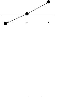
In the diagram below, the forces acting on the jth particle are shown.
T
β
α
|
T |
|
(j − 1)d |
jd |
(j + 1)d |
|
From the diagram,
Fj = T sin β − T sin α.
We make the assumption that the angles α and β are small. (The string is not stretched too much!) In this small angle approximation we have
sin α ≈ tan α and sin β ≈ tan β.
Therefore, in this small angle approximation
|
Fj |
≈ |
|
T tan β − T tan α |
||||
|
|
= T |
uj+1 − uj |
− T |
uj − uj−1 |
. |
||
|
|
d |
d |
|||||
Thus, |
d2uj |
|
|
|
|
|
|
|
m |
= |
T |
(uj+1 − 2uj + uj−1) , j = 1, 2, . . . , N. |
|||||
dt2 |
d |
|||||||
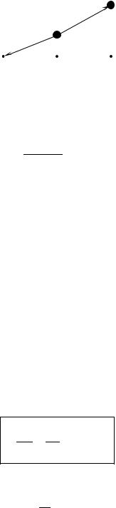
Note that these equations are valid for j = 1 and j = N when we interpret u0 uN +1 = 0. For example, for j = 1 the force F1 is determined from the diagram:
(6.1)
= 0 and
6.1. DERIVATION OF DIFFERENTIAL EQUATIONS |
69 |
T
T
0 |
d |
2d |
F = T |
(u2 − u1) |
− |
T |
u1 |
|
||
d |
d |
||||||
1 |
|
|
|||||
= |
T |
(u2 − 2u1 + u0) , u0 = 0. |
|||||
|
|||||||
d |
|||||||
Equation (6.1) is a system of N second order linear di erential equations. Thus the dimension of the vector space of solutions is 2N ; that is, it takes 2N real numbers to specify the initial conditions (N initial positions and N initial velocities). Define the N × N matrix
|
−1 2 |
−1 |
0 |
·· ·· ·· |
0 |
0 |
0 |
|
|
|||||
|
|
2 |
−1 |
0 |
0 |
|
0 |
0 |
0 |
|
|
|||
VN = |
. |
−. . |
−. |
· · · . . |
|
. |
|
|
(6.2) |
|||||
|
.. .. .. .. |
|
.. .. |
|
.. |
|
|
|
||||||
|
|
0 |
1 |
2 |
1 |
|
0 |
0 |
0 |
|
|
|||
|
|
0 |
0 |
0 |
0 |
· · · |
|
1 2 |
|
1 |
|
|
||
|
|
0 |
0 |
0 |
0 |
· · · |
− |
|
|
1 |
− |
|
|
|
|
|
|
0 |
|
2 |
|
|
|||||||
|
|
|
|
|
|
|
|
|
|
|
|
|
|
|
and the column vector u |
|
|
|
|
|
· · · |
|
|
− |
|
|
|
|
|
|
|
|
|
u1 |
|
|
|
|
|
|
|
|
|
|
|
|
|
|
|
|
|
|
|
|
|
|
|
||
u2
u = u·· |
. |
(6.3) |
|
|
N |
|
|
|
|
|
|
Then (6.1) can be written in the compact matrix form
d2u T
dt2 + md VN u = 0.
Note: We could also have written (6.1) as a first order matrix equation of the form
dx = Ax dt
(6.4)
(6.5)
where A would be a 2N × 2N matrix. However, for this application it is simpler to develop a special theory for (6.4) rather than to apply the general theory of (6.5) since the matrix manipulations with VN will be a bit clearer than they would be with A.

70 |
CHAPTER 6. WEIGHTED STRING |
6.2Reduction to an Eigenvalue Problem
Equation (6.4) is the matrix version of the harmonic oscillator equation
d2x |
+ |
k |
x = 0, |
ω02 = |
k |
. |
(6.6) |
dt2 |
|
|
|||||
|
m |
|
m |
|
|||
Indeed, we will show that (6.4) is precisely N harmonic oscillators (6.6)—once one chooses the correct coordinates. We know that solutions to (6.6) are linear combinations of
cos ω0t and sin ω0t.
Thus we “guess” that solutions to (6.4) are linear combinations of the form
cos ωt f and sin ωt f
where ω is to be determined and f is a column vector of length N . (Such a “guess” can be theoretically deduced from the theory of the matrix exponential when (6.4) is rewritten in the form (6.5).)
Thus setting
u = eiωtf ,
we see that (6.4) becomes the matrix equation
VN f = mdT ω2f .
That is, we must find the eigenvalues and eigenvectors of the matrix VN . Since VN is a real symmetric matrix, it is diagonalizable with real eigenvalues. To each eigenvalue λn, i.e.
VN fN = λnfN, n = 1, 2, . . . , N,
there will correspond a positive frequency
ωn2 = mdT λn, n = 1, 2, . . . , N,
and a solution of (6.4) of the form
uN = (an cos(ωnt) + bn sin(ωnt)) fN
where an and bn are constants. This can now be easily verified by substituting this above expression into the di erential equation. To see we have enough constants of integration we observe that we have two constants, an and bn, for each (vector) solution uN. And we have N vector solutions uN—thus 2N constants in all. We now turn to an explicit evaluation of the frequencies ωn2 —such frequencies are called normal modes.
6.3Computation of the Eigenvalues of VN
We introduce the characteristic polynomial of the matrix VN :
DN (λ) = DN = det (VN − λI) .
6.3. COMPUTATION OF THE EIGENVALUES |
71 |
Expanding the determinant DN in the last column, we see that it is a sum of two terms— each a determinant of matrices of size (N − 1) × (N − 1). One of these determinants equals (2 − λ)DN −1 and the other equals DN −2 as is seen after expanding again, this time by the last row. In this way one deduces
DN = (2 − λ)DN −1 − DN −2, N = 2, 3, 4, . . .
with
D0 = 1 and D1 = 2 − λ.
We now proceed to solve this constant coe cient di erence equation (in N ). From earlier work we know that the general solution is of the form
c1µN1 + c2µN2
where µ1 and µ2 are the roots of
µ2 − (2 − λ)µ + 1 = 0.
Solving this quadratic equation gives |
|
|
|
|
|
|
|
|
|
λ |
|
1 |
|
|
|
|
|
µ1,2 = 1 − |
± |
p(2 |
− λ)2 − 4 . |
|||||
|
|
|||||||
2 |
2 |
|||||||
It will prove convenient to introduce an auxiliary variable θ through
|
|
2 − λ = 2 cos θ, |
||||||||
A simple computation now shows |
|
|
|
|
|
|
|
|
||
|
|
|
µ1,2 = e±iθ . |
|||||||
Thus |
|
|
|
|
|
|
|
|
|
|
|
DN = c1eiN θ + c2e−iN θ . |
|||||||||
To determine c1 and c2 we require that |
|
|
|
|
|
|
||||
|
D0 = 1 |
and |
D1 = 2 − λ. |
|||||||
That is, |
|
|
|
|
|
|
|
|
|
|
|
|
c1 + c2 |
= |
1, |
|
|
||||
c1eiθ + c2e−iθ |
= |
|
2 − λ = 2 cos θ. |
|||||||
Solving for c1 and c2, |
|
|
|
|
|
|
|
|
|
|
|
|
|
|
|
|
|
eiθ |
|||
|
|
c1 |
= |
|
|
|
|
, |
|
|
|
eiθ − e−iθ |
|||||||||
|
|
c2 |
= − |
|
|
e−iθ |
||||
|
|
|
|
. |
||||||
|
eiθ − e−iθ |
|||||||||
Therefore, |
|
|
|
|
|
|
|
|
|
|
DN = |
|
1 |
ei(N +1)θ − e−i(N +1)θ |
|||||||
|
eiθ − e−iθ |
|||||||||
= |
|
sin ((N + 1)θ) |
. |
|||||||
|
|
|||||||||
|
|
sin θ |
|
|
|
|
|
|
||