

72 |
|
|
|
|
|
|
|
|
CHAPTER 6. WEIGHTED STRING |
||||
The eigenvalues of VN are solutions to |
|
|
|
|
|
|
|||||||
|
|
DN (λ) = det(VN − λI) = 0. |
|
|
|
||||||||
Thus we require |
|
|
|
|
|
|
|
|
|
|
|
|
|
|
|
|
sin ((N + 1)θ) = 0, |
|
|
|
|
||||||
which happens when |
|
|
|
|
nπ |
|
|
|
|
|
|
||
|
|
|
|
|
|
|
|
|
|
|
|||
|
θ = θn := |
|
|
|
, n = 1, 2, . . . , N. |
|
|
||||||
|
N + 1 |
|
|
||||||||||
Thus the eigenvalues of VN are |
|
|
|
|
|
|
|||||||
λn = 2 − 2 cos θn = 4 sin2(θn/2), n = 1, 2, . . . , N. |
|
(6.7) |
|||||||||||
The eigenfrequencies are |
|
|
|
|
|
|
|
|
|
|
|
|
|
ωn2 = |
T |
|
2T |
|
|
|
|
|
|
||||
|
λn = |
|
(1 − cos θn) |
|
|
|
|
|
|||||
md |
md |
md sin2 |
|
2(N + 1) |
. |
(6.8) |
|||||||
= |
md |
1 − cos N + 1 |
= |
||||||||||
|
2T |
|
|
|
|
nπ |
|
4T |
|
nπ |
|
|
|
Remark: We know there are at most N distinct eigenvalues of VN . The index n does not start at zero because this would imply θ = 0, but θ = 0—due to the presence of sin θ in the denominator of DN —is not a zero of the determinant and hence does not correspond to an eigenvalue of VN . We conclude there are N distinct eigenvalues of VN . These eigenfrequencies are also called normal modes or characteristic oscillations.
6.4The Eigenvectors
6.4.1Constructing the Eigenvectors fN
We now find the eigenvector fn corresponding to eigenvalue λn. That is, we want a column vector fN that satisfies
VN fN = 2(1 − cos θn)fN, |
n = 1, 2, . . . , N. |
|
Setting, |
|
|
fn1 |
||
fn2 |
|
|
|
·· |
|
fN = f |
, |
|
|
nN |
|
|
|
|
the above equation in component form is
−fn,j−1 + 2fn,j − fn,j+1 = 2(1 − cos θn)fn,j
with
fn,0 = fn,N +1 = 0.
6.4. THE EIGENVECTORS |
73 |
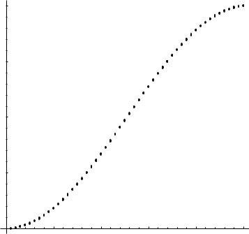
Eigenvalues for N=50 particles
4
3
2
1
n
10 |
20 |
30 |
40 |
50 |
Figure 6.1: Eigenvalues λn, (6.7), for N = 50 particles.
74 |
CHAPTER 6. WEIGHTED STRING |
This is a constant coe cient di erence equation in the j index . Assume, therefore, a solution
of the form
fn,j = eijϕ .
The recursion relation becomes with this guess
−2 cos ϕ + 2 = 2(1 − cos θn),
i.e.
ϕ = ±θn.
The fn,j will be linear combinations of e±ijθN ,
fn,j = c1 sin(jθn) + c2 cos(jθn).
We require fn,0 = fn,N +1 = 0 which implies c2 = 0.
To summarize,
V f |
= |
|
md |
2 |
|
|
|
|
|
|
|
|
|
|
ω |
f , n = 1, 2, . . . , N, |
|
|
|||||||
|
|
|
|
|||||||||
N N |
|
|
T |
n N |
|
|
|
|
|
|
|
|
|
|
|
|
|
|
|
|
|
|
|
|
|
ωn2 |
= |
|
2T |
(1 − cos θn), |
θn = |
nπ |
, |
|
||||
|
|
|
|
|||||||||
|
md |
N + 1 |
||||||||||
|
|
|
sin(θn) |
|
|
|
|
|
(6.9) |
|||
fN |
= |
sin(2θn) |
n = 1, 2, . . . , N. |
|
||||||||
|
|
· |
|
|
|
|
||||||
|
|
|
|
|
|
|
|
|
|
|
|
|
|
|
sin(N· |
θ |
) |
|
|
|
|
|
|||
|
|
|
|
|
n |
|
|
|
|
|
|
|
|
|
|
|
|
|
|
|
|
|
|
|
|
The general solution to (6.4) is
|
N |
|
|
X |
|
u(t) = |
(an cos(ωnt) + bn sin(ωnt)) fN, |
|
|
n=1 |
|
or in component form, |
|
|
N |
|
|
X |
|
|
uj (t) = |
(an cos(ωnt) + bn sin(ωnt)) sin(jθn). |
(6.10) |
n=1
Thus every oscillation of the weighted string is a sum of characteristic oscillations.
6.4.2Orthogonality of Eigenvectors
The set of eigenvectors {fN}Nn=1 forms a basis for RN since the matrix VN is symmetric. (Another reason they form a basis is that the eigenvalues of VN are distinct.) We claim the eigenvectors have the additional (nice) property that they are orthogonal, i.e.
fN · fM = 0, n 6= m,
6.5. DETERMINATION OF CONSTANTS |
75 |
where · denotes the vector dot product. The orthogonality is a direct result of the fact that VN is a symmetric matrix. Another way to prove this is to use (6.9) to compute
N |
|
X |
|
fN · fM = sin(jθn) sin(jθm). |
(6.11) |
j=1
To see that this is zero for n 6= m, we leave as an exercise to prove the trigonometric identity
N |
N + 1 |
sin |
N + 1 |
|
= |
2 (N + 1)δn,m |
|||
j=1 sin |
|||||||||
X |
|
njπ |
|
|
mjπ |
|
|
1 |
|
where δn,m is the Kronecker delta function. (One way to prove this identity is first to use the formula sin θ = (eiθ − e−iθ )/2i to rewrite the above sum as a sum of exponentials. The resulting sums will be finite geometric series.) From this identity we also get that the length of each vector, kfnk, is
kfnk = r |
|
N |
2 |
|
. |
|
|
|
+ 1 |
|
|
6.5Determination of constants an and bn
Given the initial vectors u(0) and u˙(0), we now show how to determine the constants an
and bn. At t = 0,
N
X
u(0) = anfN.
n=1
Dotting the vector fP into both sides of this equation and using the orthogonality of the eigenvectors, we see that
|
N |
N + 1 |
uj (0), p = 1, 2, . . . , N. |
(6.12) |
|
ap = N + 1 j=1 sin |
|||||
2 |
X |
|
pjπ |
|
|
Di erentiating u(t) with respect to t and then setting t = 0, we have
X
u˙(0) = ωnbnfN.
n=1
Likewise dotting fP into both sides of this equation results in
bp = N + 1 ωp |
N |
N + 1 |
u˙ j (0), p = 1, 2, . . . , N. |
(6.13) |
||
j=1 sin |
||||||
2 |
1 |
X |
|
pjπ |
|
|
If we assume the weighted string starts in an initial state where all the initial velocities are zero,
u˙ j (0) = 0,
then the solution u(t) has components
|
N |
|
|
X |
|
uj (t) = |
an cos(ωnt) sin(jθn) |
(6.14) |
n=1
76 |
CHAPTER 6. WEIGHTED STRING |
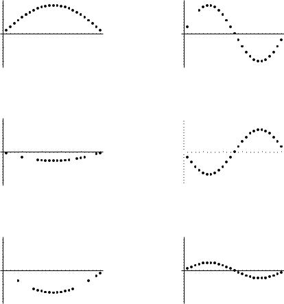
where the constants an are given by (6.12) in terms of the initial displacements uj (0). The special solutions obtained by setting all the an except for one to zero, are called the normal modes of oscillation for the weighted string. They are most interesting to graph as a function both in space (the j index) and in time (the t variable). In figures we show a “snapshot” of various normal mode solutions at various times t.
6.5. DETERMINATION OF CONSTANTS |
77 |
1
0.5
5 10 15 20 25
-0.5 -1
1
0.5

 5
5
 10 15
10 15  20
20 25
25
-0.5 -1
1
0.5

 5 10 15 20
  25 -0.5


-1
1
0.5 
j |
5 |
10 15 20 25 |
-0.5 -1
|
1 |
|
|
|
||
j |
0.5 |
|
|
|
||
|
|
|
|
|
||
-0.5 |
5 |
10 15 20 25 |
||||
|
||||||
|
|
|
|
|||
|
-1 |
|
|
|
||
1
0.5
j |
5 |
10 15 20 25 |
-0.5 -1
j
j
j
Figure 6.2: Vertical displacements uj for the two lowest (n = 1 and n = 2) normal modes are plotted as function of the horizontal position index j. Each column gives the same normal mode but at di erent times t. System is for N = 25 particles.
78 |
CHAPTER 6. WEIGHTED STRING |
1 

0.5
20 40 60 80100
-0.5 -1
1
0.5
 20 40 60 80100 -0.5


-1
1
0.5
20
 40 60
40 60
 80100
80100
-0.5 -1
|
1 |
|
|
|
j |
0.5 |
|
j |
|
|
|
|
||
-0.5 |
20 40 60 80100 |
|||
|
|
|
||
|
-1 |
|
|
|
1
0.5
j |
|
j |
20 40 60 80100 |
-0.5 -1
1
0.5
j |
|
j |
20 40 60 80100 |
-0.5
 -1
-1 
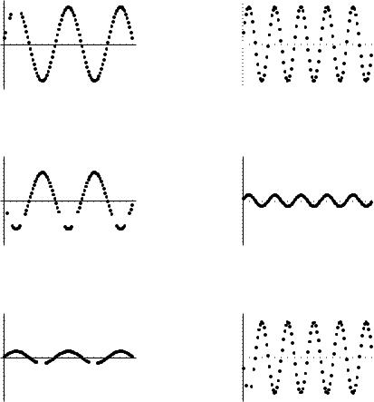
Figure 6.3: Vertical displacements uj for the two normal modes n = 5 and n = 10 are plotted as function of the horizontal position index j. Each column gives the same normal mode but at di erent times t. System is for N = 100 particles.