

CHAPTER 3. NONLINEAR STATE SPACE ESTIMATION
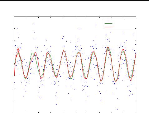
Estimating a random Sine signal with extended Kalman filter.
4 |
|
|
|
|
|
|
|
|
|
|
|
|
|
|
|
|
|
|
Measurements |
|
|
|
|
|
|
|
|
|
|
Real signal |
|
|
3 |
|
|
|
|
|
|
|
Filtered estimate |
|
|
|
|
|
|
|
|
|
|
|
|
|
2 |
|
|
|
|
|
|
|
|
|
|
1 |
|
|
|
|
|
|
|
|
|
|
0 |
|
|
|
|
|
|
|
|
|
|
−1 |
|
|
|
|
|
|
|
|
|
|
−2 |
|
|
|
|
|
|
|
|
|
|
−3 |
|
|
|
|
|
|
|
|
|
|
−4 |
|
|
|
|
|
|
|
|
|
|
0 |
50 |
100 |
150 |
200 |
250 |
300 |
350 |
400 |
450 |
500 |
Figure 3.1: Filtered estimate of the sine signal using the first order extended Kalman filter.
it gives lower error and is slightly less demanding in terms of computation power. Whether first or second order EKF should be used is ultimately up to the goal of application. If the actual signal value is of interest, which is usually the case, then one should use first order EKF, but second order one might better at predicting new signal values as the variables and a are closer to real ones on average.
3.3Unscented Kalman Filter
3.3.1 Unscented Transform
Like Taylor series based approximation presented above also the unscented transform (UT) (Julier et al., 1995; Julier and Uhlmann, 2004b; Wan and van der Merwe, 2001) can be used for forming a Gaussian approximation to the joint distribution of random variables x and y, which are defined with equations (3.1). In UT we deterministically choose a fixed number of sigma points, which capture the desired moments (at least mean and covariance) of the original distribution of x exactly. After that we propagate the sigma points through the non-linear function g and estimate the moments of the transformed variable from them.
The advantage of UT over the Taylor series based approximation is that UT is better at capturing the higher order moments caused by the non-linear transform, as
26

CHAPTER 3. NONLINEAR STATE SPACE ESTIMATION
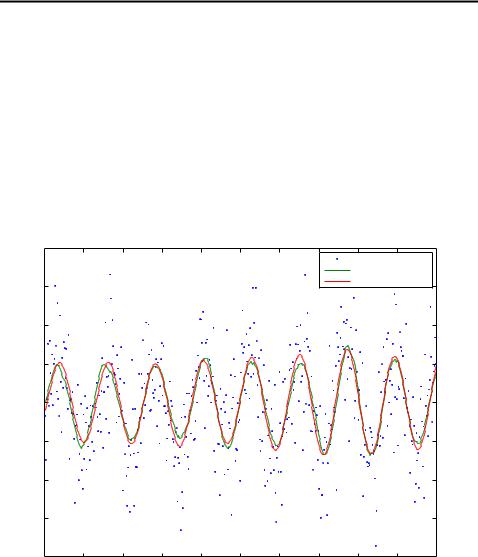
Smoothing a random Sine signal with extended Kalman (RTS) smoother.
4 |
|
|
|
|
|
|
|
|
|
|
|
|
|
|
|
|
|
|
Measurements |
|
|
|
|
|
|
|
|
|
|
Real signal |
|
|
3 |
|
|
|
|
|
|
|
Smoothed estimate |
|
|
|
|
|
|
|
|
|
|
|
|
|
2 |
|
|
|
|
|
|
|
|
|
|
1 |
|
|
|
|
|
|
|
|
|
|
0 |
|
|
|
|
|
|
|
|
|
|
−1 |
|
|
|
|
|
|
|
|
|
|
−2 |
|
|
|
|
|
|
|
|
|
|
−3 |
|
|
|
|
|
|
|
|
|
|
−4 |
|
|
|
|
|
|
|
|
|
|
0 |
50 |
100 |
150 |
200 |
250 |
300 |
350 |
400 |
450 |
500 |
Figure 3.2: Smoothed estimate of the sine signal using the extended Kalman (RTS) smoother.
Method |
RMSE[ ] |
RMSE[!] |
RMSE[a] |
RMSE[y] |
EKF1 |
0.64 |
0.53 |
0.40 |
0.24 |
ERTS1 |
0.52 |
0.31 |
0.33 |
0.15 |
ETF1 |
0.53 |
0.31 |
0.34 |
0.15 |
EKF2 |
0.34 |
0.54 |
0.31 |
0.29 |
ERTS2 |
0.24 |
0.30 |
0.18 |
0.15 |
ETF2 |
0.24 |
0.30 |
0.18 |
0.15 |
UKF |
0.59 |
0.56 |
0.39 |
0.27 |
URTS |
0.45 |
0.30 |
0.30 |
0.15 |
Table 3.1: RMSEs of estimating the random sinusoid over 100 Monte Carlo simulations.
27
CHAPTER 3. NONLINEAR STATE SPACE ESTIMATION
Smoothing a random Sine signal with extended Kalman (Two Filter) smoother.
4 |
|
|
|
|
|
|
|
|
|
|
|
|
|
|
|
|
|
|
Measurements |
|
|
|
|
|
|
|
|
|
|
Real signal |
|
|
3 |
|
|
|
|
|
|
|
Smoothed estimate |
|
|
|
|
|
|
|
|
|
|
|
|
|
2 |
|
|
|
|
|
|
|
|
|
|
1 |
|
|
|
|
|
|
|
|
|
|
0 |
|
|
|
|
|
|
|
|
|
|
−1 |
|
|
|
|
|
|
|
|
|
|
−2 |
|
|
|
|
|
|
|
|
|
|
−3 |
|
|
|
|
|
|
|
|
|
|
−4 |
|
|
|
|
|
|
|
|
|
|
0 |
50 |
100 |
150 |
200 |
250 |
300 |
350 |
400 |
450 |
500 |
Figure 3.3: Smoothed estimate of the sine signal using a combination of two extended Kalman filters.
28
CHAPTER 3. NONLINEAR STATE SPACE ESTIMATION
discussed in (Julier and Uhlmann, 2004b). Also the Jacobian and Hessian matrices are not needed, so the estimation procedure is in general easier and less error-prone.
The unscented transform can be used to provide a Gaussian approximation for the joint distribution of variables x and y of the form
y |
N |
U |
; |
CUT |
SU |
: |
(3.33) |
x |
|
m |
|
P |
CU |
|
|
The (nonaugmented) transformation is done as follows:
1.Compute the set of 2n + 1 sigma points from the columns of the matrix
p
(n + ) P:
x(0)
x(i)
x(i)
= m |
|
|
|||
= m + hp |
|
ii ; |
|
|
|
(n + ) P |
i = 1; : : : ; n |
(3.34) |
|||
= m hp |
|
ii ; |
|
|
|
(n + ) P |
i = n + 1; : : : ; 2n |
|
|||
and the associated weights: |
|
|
Wm(0) = =(n + ) |
|
|
Wc(0) = =(n + ) + (1 2 + ) |
(3.35) |
|
Wm(i) = 1=f2(n + )g; i = 1; : : : ; 2n |
|
|
Wc(i) = 1=f2(n + )g; i = 1; : : : ; 2n: |
|
|
Parameter is a scaling parameter, which is defined as |
|
|
|
= 2 (n + ) n: |
(3.36) |
The positive constants , and are used as parameters of the method. |
||
2. Propagate each of the sigma points through non-linearity as |
|
|
y(i) = g(x(i)); i = 0; : : : ; 2n: |
(3.37) |
|
3. Calculate the mean and covariance estimates for y as |
|
|
|
2n |
|
U |
Xi |
|
Wm(i) y(i) |
(3.38) |
|
|
=0 |
|
|
2n |
|
SU |
Xi |
|
Wc(i) (y(i) U ) (y(i) U )T : |
(3.39) |
|
|
=0 |
|
4. Estimate the cross-covariance between x and y as |
|
|
|
2n |
|
CU |
Xi |
|
Wc(i) (x(i) m) (y(i) U )T : |
(3.40) |
|
|
=0 |
|
29