CHAPTER 3. NONLINEAR STATE SPACE ESTIMATION

3.7Demonstration: Bearings Only Tracking

Next we review a classical filtering application (see, e.g., Bar-Shalom et al., 2001), in which we track a moving object with sensors, which measure only the bearings (or angles) of the object with respect positions of the sensors. There is a one moving target in the scene and two angular sensors for tracking it. Solving this problem is important, because often more general multiple target tracking problems can be partitioned into sub-problems, in which single targets are tracked separately at a time (Särkkä et al., 2007).

The state of the target at time step k consists of the position in two dimensional cartesian coordinates xk and yk and the velocity toward those coordinate axes, xk and yk. Thus, the state vector can be expressed as

The dynamics of the target is modelled as a linear, discretized Wiener velocity model (Bar-Shalom et al., 2001)

where q is the spectral density of the noise, which is set to q = 0:1 in the simulations. The measurement model for sensor i is defined as

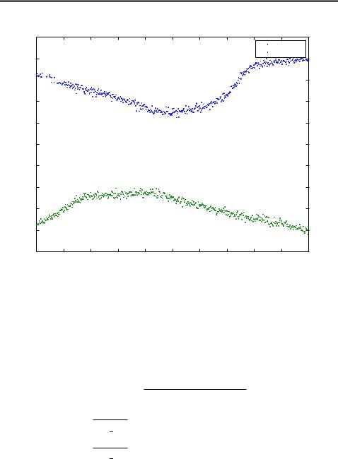
where (six; siy) is the position of sensor i and rki N(0; 2), with = 0:05 radians. In figure 3.8 we have plotted a one realization of measurements in radians

obtained from both sensors. The sensors are placed to (s1x; s1y) = ( 1; 2) and

(s2x; s2y) = (1; 1).

The derivatives of the measurement model, which are needed by EKF, can be

52

CHAPTER 3. NONLINEAR STATE SPACE ESTIMATION

Measurements from sensors in radians

2

Sensor 1

Sensor 2

1.5

1

0.5

0

−0.5

−1

−1.5

−2

−2.5

−3

Figure 3.8: Measurements from sensors (in radians) in bearings only tracking problem .

computed as

@hi(xk) = 0

@xk

@hi(xk) = 0; i = 1; 2: @yk

With these the Jacobian can written as

The non-zero second order derivatives of the measurement function are also rela-

53

CHAPTER 3. NONLINEAR STATE SPACE ESTIMATION

tively easy to compute in this model:

Thus, the Hessian matrices can be written as

(3.84) We do not list the program code for the measurement function and it’s derivatives here as they are straightforward to implement, if the previous examples have been read.

The target starts with state x0 = 0 0 1 0 , and in the estimation we set the prior distribution for the state to x0 N(0; P0), where

01

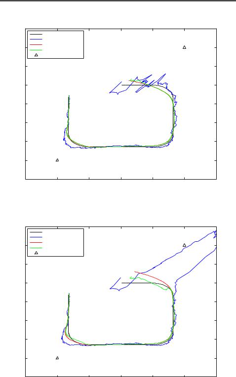
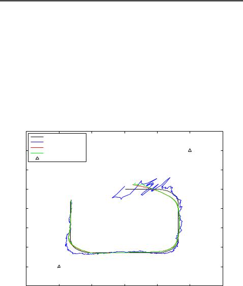
which basically means that we are fairly certain about the target’s origin, but very uncertain about the velocity. In the simulations we also give the target an slightly randomized acceleration, so that it achieves a curved trajectory, which is approximately the same in different simulations. The trajectory and estimates of it can be seen in figures 3.9, 3.10 and 3.11. As can be seen from the figures EKF1 and UKF give almost identical results while the estimates of EKF2 are clearly worse. Especially in the beginning of the trajectory EKF2 has great difficulties in getting on the right track, which is due to the relatively big uncertainty in the starting velocity. After that the estimates are fairly similar.

In table 3.3 we have listed the root mean square errors (mean of position errors) of all tested methods (same as in random sine signal example on page 25 with the addition of UTF) over 1000 Monte Carlo runs. The numbers prove the previous observations, that the EKF1 and UKF give almost identical performances. Same observations apply also to smoothers. Had the prior distribution for the starting velocity been more accurate the performance difference between EKF2 and other methods would have been smaller, but still noticeable.

54

CHAPTER 3. NONLINEAR STATE SPACE ESTIMATION

Table 3.3: RMSEs of estimating the position in Bearings Only Tracking problem over 1000 Monte Carlo runs. The Gauss–Hermite rule is of degree 3.

These observations also hold for the cubature methods. The Gauss–Hermite Kalman filter and cubature Kalman filter give practically identical results as the unscented filter.

55

CHAPTER 3. NONLINEAR STATE SPACE ESTIMATION

Filtering and smoothing result with 1st order EKF

Figure 3.9: Filtering and smoothing results of first order EKF.

Filtering and smoothing result with 2nd order EKF

Figure 3.10: Filtering and smoothing results of second order EKF.

56

CHAPTER 3. NONLINEAR STATE SPACE ESTIMATION

Filtering and smoothing result with UKF

Figure 3.11: Filtering and smoothing results of UKF

57