CHAPTER 3. NONLINEAR STATE SPACE ESTIMATION

5. Estimate the innovation covariance matrix

2n

Skjk 1 = 21n XYi;kjk 1Yi;kjk 1T y^kjk 1y^kjk 1T + Rk: i=1

6. Estimate the cross-covariance matrix

2n

Pxy;kjk 1 = 21n XXi;k 1jk 1Yi;kjk 1T mkjk 1y^kjk 1T: i=1

7. Calculate the Kalman gain term and the smoothed state mean and covariance

Kk = Pxy;kjk 1S j1

k k 1

mkjk = mkjk 1 + Kk(yk y^k

Pkjk = Pkjk 1 KkPyy;kjk 1KkT:

3.5.3 Spherical-Radial Cubature Kalman Smoother

The cubature Rauch–Tung–Striebel smoother (CRTS) algorithm (see Solin, 2010) is presented below. Assume the filtering result mean mkjk and covariance Pkjk are known together with the smoothing result p(xk+1 j y1:T ) = N(mk+1jT ; Pk+1jT ).

44

CHAPTER 3. NONLINEAR STATE SPACE ESTIMATION

3.6Demonstration: UNGM-model

To illustrate some of the advantages of UKF over EKF and augmented form UKF over non-augmented lets now consider an example, in which we estimate a model called Univariate Nonstationary Growth Model (UNGM), which is previously used as benchmark, for example, in Kotecha and Djuric (2003) and Wu et al. (2005). What makes this model particularly interesting in this case is that its highly nonlinear and bimodal, so it is really challenging for traditional filtering techniques. We also show how in this case the augmented version of UKF gives better performance than the nonaugmented version. Additionally the Cubature (CKF) and Gauss–Hermite Kalman filter (GHKF) results are also provided for comparison.

The dynamic state space model for UNGM can be written as

where un N(0; u2) and vn N(0; u2). In this example we have set the parameters to u2 = 1, v2 = 1, x0 = 0:1, = 0:5, = 25, = 8, and N = 500. The cosine term in the state transition equation simulates the effect of time-varying

noise.

In this demonstration the state transition is computed with the following function:

function x_n = ungm_f(x,param)

n = param(1);

x_n = 0.5*x(1,:) + 25*x(1,:)./(1+x(1,:).*x(1,:)) + 8*cos(1.2*(n-1)); if size(x,1) > 1 x_n = x_n + x(2,:); end

where the input parameter x contains the state on the previous time step. The current time step index n needed by the cosine term is passed in the input parameter param. The last three lines in the function adds the process noise to the state

45

CHAPTER 3. NONLINEAR STATE SPACE ESTIMATION

component, if the augmented version of the UKF is used. Note that in augmented UKF the state, process noise and measurement noise terms are all concatenated together to the augmented variable, but in URTS the measurement noise term is left out. That is why we must make sure that the functions we declare are compatible with all cases (nonaugmented, augmented with and without measurement noise). In this case we check whether the state variable has second component (process noise) or not.

Similarly, the measurement model function is declared as

function y_n = ungm_h(x_n,param)

y_n = x_n(1,:).*x_n(1,:) ./ 20;

if size(x_n,1) == 3 y_n = y_n + x_n(3,:); end

The filtering loop for augmented UKF is as follows:

for k = 1:size(Y,2)

[M,P,X_s,w] = ukf_predict3(M,P,f_func,u_n,v_n,k); [M,P] = ukf_update3(M,P,Y(:,k),h_func,v_n,X_s,w,[]); MM_UKF2(:,k) = M;

PP_UKF2(:,:,k) = P; end

The biggest difference in this in relation to other filters is that now the predict step returns the sigma points (variable X_s) and their weigths (variable w), which must be passed as parameters to update function.

To compare the EKF and UKF to other possible filtering techniques we have also used a bootstrap filtering approach (Gordon et al., 1993), which belongs to class of Sequential Monte Carlo (SMC) methods (also known as particle filters). Basically the idea in SMC methods that is during each time step they draw a set of weighted particles from some appropriate importance distribution and after that the moments (that is, mean and covariance) of the function of interest (e.g. dynamic function in state space models) are estimated approximately from drawn samples. The weights of the particles are adjusted so that they are approximations to the relative posterior probabilities of the particles. Usually also a some kind of resampling scheme is used to avoid the problem of degenerate particles, that is, particles with near zero weights are removed and those with large weights are duplicated. In this example we used a stratified resampling algorithm (Kitagawa, 1996), which is optimal in terms of variance. In bootstrap filtering the dynamic model p(xkjxk 1) is used as importance distribution, so its implementation is really easy. However, due to this a large number of particles might be needed for the filter to be effective. In this case 1000 particles were drawn on each step. The implementation of the bootstrap filter is commented out in the actual demonstration script (ungm_demo.m), because the used resampling function (resampstr.m) was originally provided in MCMCstuff toolbox (Vanhatalo and Vehtari, 2006), which can be found at http://www.lce.hut.fi/research/mm/mcmcstuff/.

46

CHAPTER 3. NONLINEAR STATE SPACE ESTIMATION

UKF2 filtering result

EKF filtering result

Bootstrap filtering result

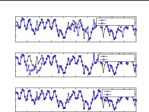
Figure 3.4: First 100 samples of filtering results of EKF, augmented form UKF and bootstrap filter for UNGM-model.

In figure 3.4 we have plotted the 100 first samples of the signal as well as the estimates produced by EKF, augmented form UKF and bootstrap filter. The bimodality is easy to see from the figure. For example, during samples 10 25 UKF is able to estimate the correct mode while the EKF estimates it wrong. Likewise, during steps 45 55 and 85 95 UKF has troubles in following the correct mode while EKF is more right. Bootstrap filter on the other hand tracks the correct mode on almost ever time step, although also it produces notable errors.

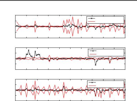
In figure 3.5 we have plotted the absolute errors and 3 confidence intervals of the previous figures filtering results. It can be seen that the EKF is overoptimistic in many cases while UKF and boostrap filter are better at telling when their results are unreliable. Also the lower error of bootstrap filter can be seen from the figure. The bimodality is also easy to notice on those samples, which were mentioned above.

The make a comparison between nonaugmented and augmented UKF we have plotted 100 first samples of their filtering results in figure 3.6. Results are very surprising (although same as in Wu et al. (2005)). The reason why nonaugmented UKF gave so bad results is not clear. However, the better performance of augmented form UKF can be explained by the fact, that the process noise is taken into account more effectively when the sigma points are propagated through nonlinearity. In this case it seems to be very crucial, as the model is highly nonlinear and multi-modal.

47

CHAPTER 3. NONLINEAR STATE SPACE ESTIMATION

UKF2 error

EKF error

Bootstrap filtering error

Figure 3.5: Absolute errors of and 3 confidence intervals of EKF, augmented form UKF and bootstrap in 100 first samples.

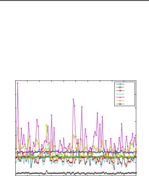
Lastly in figure 3.7 we have plotted the mean square errors of each tested methods of 100 Monte Carlo runs. Average of those errors are listed in table 3.2. Here is a discussion for the results:

•It is surprising that the nonaugmented UKF seems to be better than EKF, while in above figures we have shown, that the nonaugmented UKF gives very bad results. Reason for this is simple: the variance of the actual signal is approximately 100, which means that by simply guessing zero we get better performance than with EKF, on average. The estimates of nonaugmented UKF didn’t variate much on average, so they were better than those of EKF, which on the other hand variated greatly and gave huge errors in some cases. Because of this neither of the methods should be used for this problem, but if one has to choose between the two, that would be EKF, because in some cases it still gave (more or less) right answers, whereas UKF were practically always wrong.

•The second order EKF were also tested, but that diverged almost instantly, so it were left out from comparison.

•Augmented form UKF gave clearly the best performance from the tested Kalman filters. As discussed above, this is most likely due to the fact that the process noise terms are propagated through the nonlinearity, and hence

48

CHAPTER 3. NONLINEAR STATE SPACE ESTIMATION

UKF1 filtering result

UKF2 filtering result

Figure 3.6: Filtering results of nonaugmented UKF (UKF1) and augmented UKF (UKF2) of 100 first samples.

49

CHAPTER 3. NONLINEAR STATE SPACE ESTIMATION

Table 3.2: MSEs of estimating the UNGM model over 100 Monte Carlo simulations.

odd-order moment information is used to obtain more accurate estimates. The usage of RTS smoother seemed to improve the estimates in general, but oddly in some cases it made the estimates worse. This is most likely due to the multi-modality of the filtering problem.

•The Gauss–Hermite method performed rather well in both filtering and smoothing. This was mostly due to the degree of approximation as the rule entailed 10 sigma points.

•The cubature Kalman filter gave results close to the UKF variants, which is to no surprise as the filter uses similar sigma points.

•Bootstrap filtering solution was clearly superior over all other tested methods. The results had been even better, if greater amount of particles had been used.

The reason why Kalman filters didn’t work that well in this case is because Gaussian approximations do not in general apply well for multi-modal cases. Thus, a particle filtering solution should be preferred over Kalman filters in such cases. However, usually the particle filters need a fairly large amount of particles to be effective, so they are generally more demanding in terms of computational power than Kalman filters, which can be a limiting factor in real world applications. The errors, even with bootstrap filter, were also relatively large, so one must be careful when using the estimates in, for example, making financial decisions. In practice this means that one has to monitor the filter’s covariance estimate, and trust the state estimates and predictions only when the covariance estimates are low enough, but even then there is a change, that the filter’s estimate is completely wrong.

50

CHAPTER 3. NONLINEAR STATE SPACE ESTIMATION

MSE of different methods with 100 Monte Carlo runs

Figure 3.7: MSEs of different methods in 100 Monte Carlo runs.

51