CHAPTER 3. NONLINEAR STATE SPACE ESTIMATION

3.8Demonstration: Reentry Vehicle Tracking

Next we review a challenging filtering problem, which was used in Julier and Uhlmann (2004b) to demonstrate the performance of UKF. Later they released few corrections to the model specifications and simulation parameters in Julier and Uhlmann (2004a).

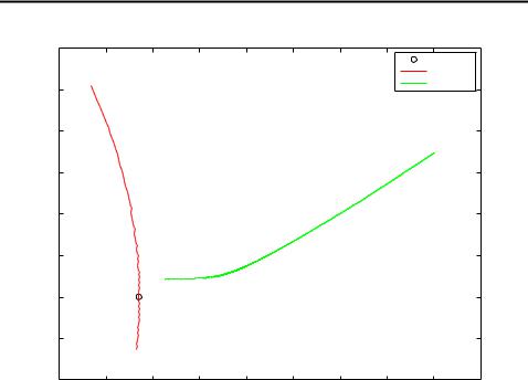
This example conserns a reentry tracking problem, where radar is used for tracking a space vehicle, which enters the atmosphere at high altitude and very high speed. Figure 3.12 shows a sample trajectory of the vehicle with respect to earth and radar. The dynamics of the vehicle are affected with three kinds of forces: aerodynamic drag, which is a function of vehicle speed and has highly nonlinear variations in altitude. The second type of force is gravity, which causes the vehicle to accelerate toward the center of the earth. The third type of forces are random buffeting terms. The state space in this model consists of vehicles position (x1 and x2), its velocity (x3 and x4) and a parameter of its aerodynamic properties (x5). The dynamics in continuous case are defined as (Julier and Uhlmann, 2004b)

x4(t) = D(t)x4(t) + G(t)x2(t) + v2(t) x5(t) = v3(t);

where w(t) is the process noise vector, D(t) the drag-related force and G(t) the gravity-related force. The force terms are given by

p

where R(t) = x21(t) + x22(t) is the vehicle’s distance from the center of the earth

p

and V (t) = x23(t) + x24(t) is the speed of the vehicle. The constants in previous definition were set to

0 = 0:59783

H0 = 13:406

(3.88)

Gm0 = 3:9860 105 R0 = 6374:

To keep the implementation simple the continuous-time dynamic equations were

58

CHAPTER 3. NONLINEAR STATE SPACE ESTIMATION

discretized using a simple Euler integration scheme, to give

x4(k + 1) = x4(k) + t(D(k)x4(k) + G(k)x2(k)) + w2(k) x5(k + 1) = x5(k) + w3(k);

where the step size between time steps was set to t = 0:1s. Note that this might be too simple approach in real world applications due to high nonlinearities in the dynamics, so more advanced integration scheme (such as Runge-Kutta) might be more preferable. The discrete process noise covariance in the simulations was set to

The lower right element in the covariance was initially in Julier and Uhlmann (2004b) set to zero, but later in Julier and Uhlmann (2004a) changed to 10 6 to increase filter stability.

The non-zero derivatives of the discretized dynamic equations with respect to

59

CHAPTER 3. NONLINEAR STATE SPACE ESTIMATION

state variables are straightforward (although rather technical) to compute:

where the (non-zero) derivatives of the force, position and velocity related terms

60

CHAPTER 3. NONLINEAR STATE SPACE ESTIMATION

The prior distribution for the state was set to multivariate Gaussian, with mean and covariance (same as in Julier and Uhlmann (2004b))

0 1

6500:4

B349:14 C

BC m0 = B 1:8093C

BC @ 6:7967A

0

In the simulations the initial state were drawn from multivariate Gaussian with

61

CHAPTER 3. NONLINEAR STATE SPACE ESTIMATION

mean and covariance

0 1

6500:4

B349:14 C

BC m0 = B 1:8093C

BC @ 6:7967A

that is, vehicle’s aerodynamic properties were not known precisely beforehand. The radar, which is located at (sx; sy) = (R0; 0), is used to measure the range

rk and bearing k in relation to the vehicle on time step k. Thus, the measurement model can be written as

where the measurement noise processes q1(k) and q2(k) are Gaussians with zero means and standard deviations r = 10 3km and = 0:17mrad, respectively. The derivatives of k with respect to state variables can computed with equations (3.81). For rk the derivatives can be written as

In the table 3.4 we have listed the RMS errors of position estimates with tested methods, which were

•EKF1: first order extended Kalman filter.

•ERTS: first order Rauch-Tung-Striebel smoother.

•UKF: augmented form unscented Kalman filter.

•URTS1: unscented Rauch-Tung-Striebel smoother with non-augmented sigma points.

•URTS2: unscented Rauch-Tung-Striebel smoother with augmented sigma points.

62

CHAPTER 3. NONLINEAR STATE SPACE ESTIMATION

Figure 3.12: Sample vehicle trajectory, earth and position of radar in Reentry Vehicle Tracking problem.

• UTF: unscented Forward-Backward smoother.

Extended Forward-Backward smoother was also tested, but it produced in many cases divergent estimates, so it was left out from comparison. Second order EKF was also left out, because evaluating the Hessians would have taken too much work while considering the fact, that the estimates might have gotten even worse.

From the error estimates we can see, that EKF and UKF — and the other methods as well — give almost identical performances, altough in the article (Julier and Uhlmann, 2004b) UKF was clearly superior over EKF. The reason for this might be the fact that they used numerical approximations (central differences) for calculating the Jacobian in EKF rather than calculating the derivatives in closed form, as was done in this demonstration.

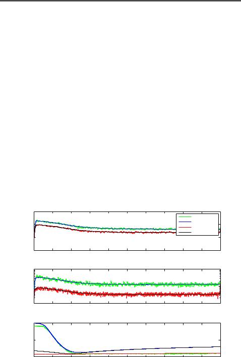
In figure 3.13 we have plotted the mean square errors and variances in estimating x1, x3 and x5 with EKF and ERTS over 100 Monte Carlo runs. It shows that using smoother always gives better estimates for positions and velocities, but for x5 the errors are practically the same after 45 seconds. This also shows that both methods are pessimistic in estimating x5, because variances were bigger than the true errors. Figures for x2 and x4 are not shown, because they are very similar to the ones of x1 and x3. Also by using UKF and URTS the resulting figures were in practically identical, and therefore left out.

63

CHAPTER 3. NONLINEAR STATE SPACE ESTIMATION

Table 3.4: Average RMSEs of estimating the position in Reentry Vehicle Tracking problem over 100 Monte Carlo runs. The Gauss–Hermite rule is of degree 3.

Figure 3.13: MSEs and variances in estimating of x1, x3 and x5 using EKF and ERTS over 100 Monte Carlo runs.

64