CHAPTER 4. MULTIPLE MODEL SYSTEMS

still provide sufficient accuracy with suitable models. filter based IMM filter for estimating more models, but that approach is not currently

The prediction and update steps of IMM-EKF is provided by functions eimm_predict and eimm_update, and smoothing can be done with function eimm_smooth. The corresponding functions for IMM-UKF are uimm_predict, uimm_update and uimm_smooth.

4.2.1 Demonstration: Coordinated Turn Model

A common way of modeling a turning object is to use the coordinated turn model (see, e.g., Bar-Shalom et al., 2001). The idea is to augment the state vector with a turning rate parameter !, which is to be estimated along with the other system parameters, which in this example are the position and the velocity of the target. Thus, the joint system vector can be expressed as

The dynamic model for the coordinated turns is

Fk

where vk N(0; !2 ) is univariate white Gaussian process noise for the turn rate parameter. This model is, despite the matrix form, non-linear. Equivalently, the dynamic model can be expressed as a set of equations

The source code of the turning model can found in the m-file f_turn.m. The inverse dynamic model can be found in the file f_turn_inv.m, which basically calculates the dynamics using the inverse Fk in eq. (4.65) as it’s transition matrix.

79

CHAPTER 4. MULTIPLE MODEL SYSTEMS

To use EKF in estimating the turning rate !k the Jacobian of the dynamic model must be computed, which is given as

@yk+1 = t cos(!k t)xk t sin(!k t)yk: @!k

(4.68)

The source code for calculating the Jacobian is located in the m-file f_turn_dx.m. Like in previous demonstration we simulate the system 200 time steps with

step size t = 0:1. The movement of the object is produced as follows:

•Object starts from origo with velocity (x; y) = (1; 0).

•At 4s object starts to turn left with rate ! = 1.

•At 9s object stops turning and moves straight for 2 seconds with a constant total velocity of one.

•At 11s objects starts to turn right with rate ! = 1.

•At 16s object stops turning and moves straight for 4 seconds with the same velocity.

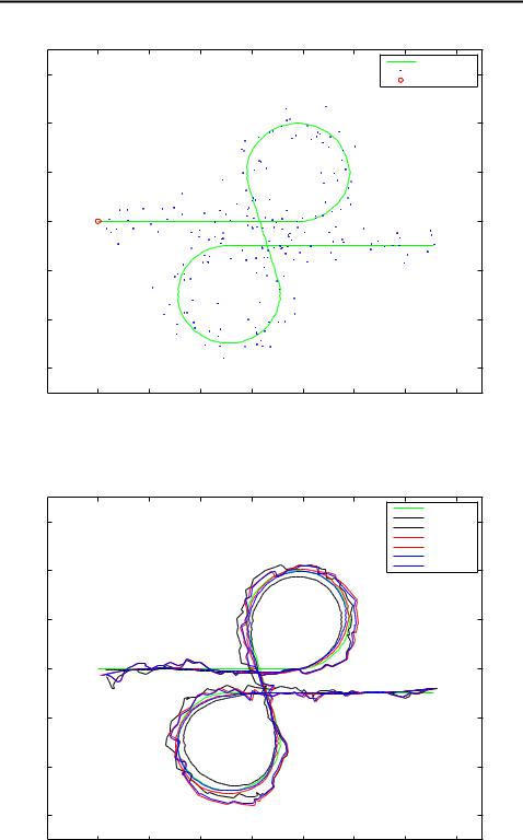
The resulting trajectory is plotted in figure 4.5. The figure also shows the measurements, which were made with the same model as in the previous example, that is, we observe the position of the object directly with the additive noise, whose variance in this case is set to r2 = 0:05.

In the estimation we use the following models:

1.Standard Wiener process velocity model (see, for example, section 2.2.9) with process noise variance q1 = 0:05, whose purpose is to model the relatively slow turns. This model is linear, so we can use the standard Kalman filter for estimation.

80

CHAPTER 4. MULTIPLE MODEL SYSTEMS

2.A combination of Wiener process velocity model and a coordinated turn model described above. The variance of the process noise for the velocity model is set to q2 = 0:01 and for the turning rate parameter in the turning model to q! = 0:15. The estimation is now done with both the EKF and UKF based IMM filters as the turning model is non-linear. However, as the measurement model is linear, we can still use the standard IMM filter update step instead of a non-linear one. In both cases the model transition

probability matrix is set to

and the prior model probabilities are

model (in case of ! = 0)

In software code the prediction step of IMM-EKF can be done with the function

call

[x_p,P_p,c_j] = eimm_predict(x_ip,P_ip,mu_ip,p_ij,ind, ...

dims,A,a_func,a_param,Q);

which is almost the same as the linear IMM-filter prediction step with the exception that we must now also pass the function handles of the dynamic model and it’s Jacobian as well as their possible parameters to the prediction step function. In above these are the variables A, a_func and a_param which are cell arrays containing the needed values for each model. If some of the used models are linear (as is the case now) their elements of the cell arrays a_func and a_param are empty, and A contains the dynamic model matrices instead of Jacobians. The prediction step function of IMM-UKF has exactly the same interface.

The EKF based IMM smoothing can be done with a function call

[SMI,SPI,SMI_i,SPI_i,MU_S] = eimm_smooth(MM,PP,MM_i,PP_i,MU,p_ij, ...

mu_0j,ind,dims,A,ia_func, ...

a_param,Q,R,H,h_func,h_param,Y);

where we pass the function handles of inverse dynamic models (variable ia_func) for the backward time IMM filters as well as Jacobians of the dynamic models (A) and their parameters (a_param), which all are cell arrays as in the filter described above. Sameway we also pass the handles to the measurement model functions (h_func) and their Jacobians (H) as well as their parameters (h_param). UKF based IMM smoothing is done exactly the same.

In figure 4.6 we have plotted the filtered and smoothed estimates produced all the tested estimation methods. It can be seen that the estimates produced by IMMEKF and IMM-UKF are very close on each other while IMM-UKF still seems to

81

CHAPTER 4. MULTIPLE MODEL SYSTEMS

Table 4.2: Average MSEs of estimating the position in Tracking Object with Simple Manouvers example over 100 Monte Carlo runs.

be a little closer to the right trajectory. The estimates of standard KF differ more from the estimates of IMM-EKF and IMM-UKF and seem to have more problems during the later parts of turns. Smoothing improves all the estimates, but in the case of KF the estimates are clearly oversmoothed.

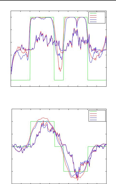
The estimates for probability of model 2 produced by IMM-EKF and IMMUKF are plotted in figure 4.7. The filtered estimates seem to be very close on each other whereas the smoothed estimates have little more variation, but neither one of them don’t seem to be clearly better. The reason why both methods give about 50% probability of model 2 when the actual model is 1 can be explained by the fact that the coordinated turn model actually contains the velocity model as it’s special case when ! = 0. The figure 4.7 shows the estimates of the turn rate parameter with both IMM filters and smoothers, and it can be seen that smoothing improves the estimates tremendously. It is also easy to see that in some parts IMM-UKF gives a little better performance than IMM-EKF.

In table 4.2 we have listed the average MSEs of position estimates produced by the tested methods. It can be seen, that the estimates produced by IMM-EKF and IMM-UKF using the combination of a velocity and a coordinated turn model are clearly better than the ones produced by a standard Kalman filter using the velocity model alone. The performance difference between IMM-EKF and IMM-UKF is also clearly noticable in the favor of IMM-UKF, which is also possible to see in figure 4.6. The effect of smoothing to estimation accuracy is similar in all cases.

4.2.2Demonstration: Bearings Only Tracking of a Manouvering Target

We now extend the previous demonstration by replacing the linear measurement model with a non-linear bearings only measurement model, which were reviewed in section 2.2.9. The estimation problem is now harder as we must use a non-linear version of IMM filter update step in addition to the prediction step, which was used in the previous demonstration.

The trajectory of the object is exactly the same as in the previous example. The sensors producing the angle measurements are located in (s1x; s1y) = ( 0:5; 3:5),

82

CHAPTER 4. MULTIPLE MODEL SYSTEMS

Figure 4.5: Object’s trajectory and a sample of measurements in the Coordinated turn model demonstration.

Figure 4.6: Position estimates in the Coordinated turn model demonstration.

83

CHAPTER 4. MULTIPLE MODEL SYSTEMS

Figure 4.7: Estimates for model 2’s probability in Coordinated turn model demon-

Figure 4.8: Estimates of the turn rate parameter !k in the Coordinated turn model demonstration.

84

CHAPTER 4. MULTIPLE MODEL SYSTEMS

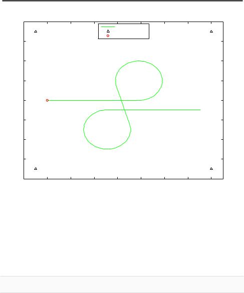
Figure 4.9: Object’s trajectory and positions of the sensors in Bearings Only Tracking of a Manouvering Target demonstration.

(s2x; s2y) = ( 0:5; 3:5), (s3x; s3y) = (7; 3:5) and (s4x; s4y) = (7; 3:5). The trajectory and the sensor positions are shown in figure 4.9. The standard deviation of the

measurements is set to = 0:1 radians, which is relatively high. The function call of IMM-EKF update step is of form

[x_ip,P_ip,mu_ip,m,P] = eimm_update(x_p,P_p,c_j,ind,dims, ...

Y(:,i),H,h_func,R,h_param);

which differs from the standard IMM filter update with the additional parameters h and h_param, which contain the handles to measurement model functions and their parameters, respectively. Also, the parameter H now contains the handles to functions calculating the Jacobian’s of the measurement functions. In IMM-UKF the update function is specified similarly.

The position of the object is estimated with the following methods:

•EKF and EKS: Extended Kalman filter and (RTS) smoother using the same Wiener process velocity model as in the previous demonstration in the case standard Kalman filter.

•UKF and UKS: Unscented Kalman filter and (RTS) smoother using the same model as the EKF.

85

CHAPTER 4. MULTIPLE MODEL SYSTEMS

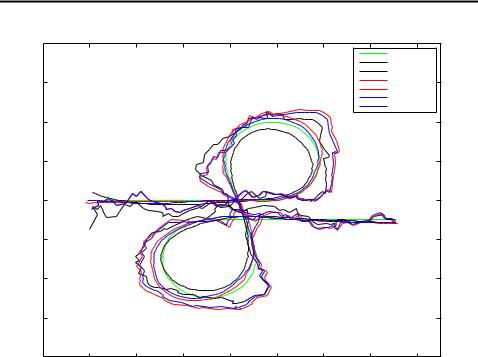
Figure 4.10: Filtered and smoothed estimates of object’s position using all the tested methods in Bearings Only Tracking of a Manouvering Target demonstration.

•IMM-EKF and IMM-EKS: EKF based IMM filter and smoother using the same combination of Wiener process velocity model and a coordinated turn model as was used in the previous demonstration in the case of IMM-EKF and IMM-UKF.

•IMM-UKF and IMM-UKS: UKF based IMM filter and smoother using the same models as IMM-EKF.

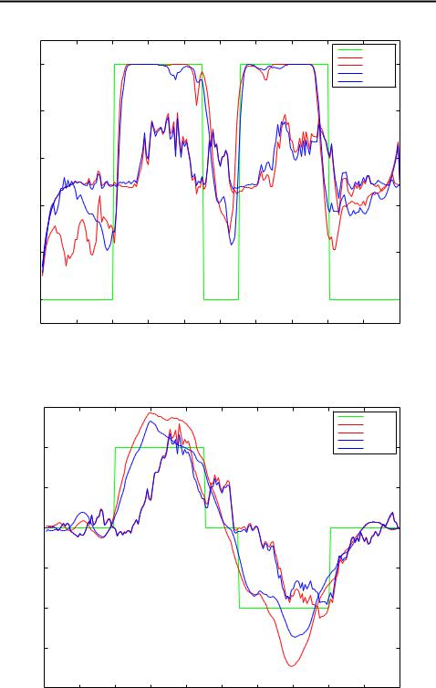
A sample of trajectory estimates are plotted in figure 4.10. The estimates are clearly more inaccurate than the ones in the previous section. In figure 4.11 we have plotted the estimates of model 2’s probability for IMM-EKF and IMM-UKF. The figure look very similar to the one in the previous demonstration, despite the non-linear and more noisy measurements. Also the turn rate estimates, which are plotted in figure 4.12, are very similar to the ones in the previous section with exception that now the difference between the smoothed estimates of IMM-EKF and IMM-UKF is bigger.

In table 4.3 we have listed the average mean square errors of position estimates over 100 Monte Carlo runs. It can be observed that the estimates of EKF and UKF are identical in practice, which is to be expected from Bearings Only Tracking demonstration. The difference between IMM-UKF and IMM-EKF has grown in the favor of IMM-UKF, whereas the accuracy of IMM-EKF is now more close to

86

CHAPTER 4. MULTIPLE MODEL SYSTEMS

Figure 4.11: Estimates for model 2’s probability in Bearings Only Tracking of a Manouvering Target demonstration.

Figure 4.12: Estimates for the turn rate parameter !k in Bearings Only Tracking of a Manouvering Target demonstration

87

CHAPTER 4. MULTIPLE MODEL SYSTEMS

Table 4.3: Average MSEs of estimating the position in Bearings Only Tracking of a Manouvering Target example over 100 Monte Carlo runs.

the ones of EKF and UKF. On the other hand the smoothed estimates of IMM-UKF and IMM-EKF are still very close to one another, and are considerably better than the smoothed estimates of EKF and UKF.

It should be noted that the performance of each tested method could be tuned by optimizing their parameters (e.g. variance of process noise of dynamic models, values of model transition matrix in IMM etc.) more carefully, so the performance differences could change radically. Still, it is clear that IMM filter does actually work also with (atleast some) non-linear dynamic and measurement models, and should be considered as a standard estimation method for multiple model systems. Also, one should prefer IMM-UKF over IMM-EKF as the performance is clearly (atleast in these cases) better, and the implementation is easier, as we have seen in the previous examples.

88