PHASE TRANSITION (lectures)

ФИЗИЧЕСКИЙ ФАКУЛЬТЕТ КАЗАНСКИЙ ГОСУДАРСТВЕННЫЙ УНИВЕРСИТЕТ

Хасанов Б.М.

PHASE TRANSITIONS

ФАЗОВЫЕ ПЕРЕХОДЫ

(краткие конспекты лекций)

Казань 2010

Contents

3

Phase transitions

Phase transitions

In nature there are many systems that exist in different phases. Examples are solid-liquid-gas, magnetic, ferroelectric, and other ·systems. Here we will discuss transitions between such phases.

When two phases, say 1 and 2 are in contact with each other, there is an interface separating the phases. In equilibrium, the chemical potentials of both phases in contact are equal,

and the two phases coexist (See Figure 1.1).

first order. Dashed portions represent unstable states. In figure (b) the transition is continuous and the two phases meet in the critical point CP.

Classification of phase transitions

As one of the parameters (e.g., the temperature) is varied in such a way that the coexistence line is crossed, the system undergoes a phase transition between the two phases. At the phase transition a derivative of the free energy (or some other

4

Phase transitions

thermodynamic potential) is discontinuous. The free energy (thermodynamic potential) becomes non-analytic in this point. The transition can be either first order or continuous.

(a) First-order phase transitions. The conditions for first-order phase transitions are that the chemical potentials are equal,

and that their derivatives are different,

so that the chemical potentials or the free energies cross at the transition. The phase with the lower chemical potential is stable and the other phase is metastable. An example of a first-order phase transition is the liquid-gas transition.

(b) Continuous phase transitions. A transition is continuous when the chemical potentials of both phases are equal and when their first derivatives are also equal,

so that the chemical potentials or the free energies have a common tangent at the transition. There is no latent heat in this type of transition.

Instead of continuous transitions, some authors write about second, third, and higher order transitions, depending on which derivative of the chemical potential diverges or becomes discontinuous. This classification is somewhat arbitrary, therefore we will distinguish only between the continuous and first-order transitions.

Order parameter

As an example, let us consider a simple ferromagnetic material. At high temperatures, there is no magnetization and the system is rotationally invariant. At low

5

Phase transitions

temperatures, when spontaneous magnetization occurs, the magnetization direction define a preferred direction in space, destroying the rotational invariance. We call this spontaneous symmetry breaking and it takes place at the critical temperature (for ferromagnets it is the Curie point). Since a symmetry is either absent or present, the two phases must be described by different functions of thermodynamic variables, which cannot be continued analytically across the critical point.

Because of the reduction in symmetry, an additional parameter is needed to describe the thermodynamics of the low-temperature phase. This parameter is called the order parameter. It is usually an extensive thermodynamic variable. In the case of ferromagnets, the order parameter is the thermal average of the (total) magnetization, hMi. For the gas-liquid transition, the order parameter is either the volume or the density difference between the two phases. Notice that the density is not an extensive quantity. Notice also that there is no obvious symmetry change in the gas-liquid transition.

The basic idea of phase transitions is that near the critical point, the order parameter is the only relevant thermodynamic quantity.

Some examples of the order parameters and conjugate field are given in the following table:

Critical point

1. Liquid-gas transitions. In Figure 1.2 a typical phase diagram of a solid- liquid-gas system in the P −T plane at constant V and N is shown. Here we would like to concentrate on the liquid-gas transition. The liquid and the gas phases coexist along a line where the transition between these two phases is first order.

6

Phase transitions

Figure 1.3: Phase diagram of a ferromagnet.

7

Phase transitions

If T is increased, the coexistence line terminates in the critical point, where the transition between the two phases is continuous. Beyond the critical point, there is no transition between the two phases, there is no singularity in any physical quantity upon going from one phase to the other. It is also instructive to consider the isotherms in the P − ρ plane at constant T and N, see Fig. 1.2. At low temperature, there is a large difference between the gas and liquid densities, ρG and ρL, but as the critical temperature is approached, this difference tends to zero. The existence of a quantity that is non-zero below the critical temperature and zero above it, is a common feature of critical points in a variety of different physical systems. ρL − ρG is the order parameter for the liquid-gas critical point.

2.Ferromagnets. A typical phase diagram of a ferromagnet is shown in Fig.

1.3.The order parameter is the magnetization M, i.e., the total magnetic moment. At low temperature, M is ordered either ”up” or ”down”, depending on the external field H. When H changes sign, the system undergoes a first-order phase transition (bold line) in which the magnetization changes its direction discontinuously [Fig. 1.3]. As T is increased, the critical point is reached, at which M changes continuously upon variation of H but its derivative with respect to H, i.e., the susceptibility diverges. At still higher T , there is no phase transition, the spins are simply disordered, this is the paramagnetic region.

Critical exponents

In this section the behaviour of the thermodynamic quantities near the critical point is discussed. We suppose that very near the critical point, any thermodynamic quantity can be decomposed into a ”regular” part, which remains finit (not necessarily continuous) and a ”singular part” that can be divergent or have divergent derivatives. The singular part is assumed to be proportional to some power of |T − TC | (or p − pc).

Definition of the critical exponents. For clarity, we will defin the critical exponents on a ferromagnet. However, their definition will be general and will be valid for arbitrary system that undergoes a continuous phase transition. The most important critical exponents are:

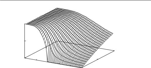
β = Order parameter exponent. When H = 0, the magnetization M in a ferromagnet is a decreasing function of T and vanishes at TC (See Fig. 1.4).

For T very close to (but below) TC , M can be written as

8

Phase transitions

M

Figure 1.4: Order parameter vs. temperature and field

β is the order parameter exponent which describes the behaviour of M near TC . Here and later, means ”the singular part is proportional to”.

δ = Exponent of the critical isotherm. When T = TC , M vanishes for H = 0 but increases very rapidly if H increases. For small H, the singular part of M is proportional to:

where δ > 1.

γ = Susceptibility exponent. As TC is approached either from above or from below, the susceptibility diverges. The divergence is described with the exponent

Notice that the exponent γ is the same for T > TC and T < TC whereas the proportionality constants are different.

α = Specific heat exponent. The specific heat at constant volume (for ferromagnetic systems one has to take H =0 )has a singularity at TC. This singularity is described by the exponent α:

As usually, the exponent α is the same for T > TC and T < TC whereas the proportionality constants are different.

ν= Correlation length exponent. As already mentioned, the correlation length

ξis a temperaturedependent quantity. As we shall see later, ξ diverges at the

9

Phase transitions

η = Correlation function exponent at the critical isotherm. At TC , ξ diverges and the correlation function decays as a power law of r,

where d is the dimensionality of the system.

Scaling. As the name suggests, the scaling has something to do with the change of various quantities under a change of length scale. Important scaling laws concerning the thermodynamic functions can be derived from the simple (but strong) assumption that, near the critical point, the correlation length ξ is the only characteristic length of the system, in terms of which all other lengths must be measured. This is the scaling hypothesis.

With the aid of the scaling hypothesis we are able to get relations between the critical exponents. The most common scaling relations are:

so that only two of the above exponents are independent. The last four equations are called the scaling laws. We shall prove some of the scaling laws later.

Universality. Some quantities depend on the microscopic details of the system. Examples of such quantities are:

-The critical temperature depends on the strength of interaction.

-The proportionality constants (e.g., for the temperature dependence of the magnetization) also depend on the microscopic properties of the system.

On the other hand, the critical exponents and the functional form of the equation of state, of the correlation functions, etc. are independent of many details of the system. They depend only on global features, such as:

-The spatial dimensionality,

-symmetry (isotropic, uniaxial, planar,...), ... .

Systems that have the same critical exponents and the same functional form of the equation of state, etc, belong to the same universality class. For example,

10