

PHASE TRANSITION (lectures)
.pdfPhase transitions
Momentum-space renormalization group
RG methods in momentum space are much more powerful and more widely used than their counterparts in real space. The problem is only that they are much more complicated than the real-space prototype examples. We shall define the RG transformation for the Landau model, that means that we shall now use continuous instead of discrete spin variables. The main reason is that discrete spins become essentially continuous after (block-spin) transformations.
We start with the free energy of the form:
H(h, m(r)) = ZV |
dd~r |
1 |
g|rm(r)|2 − m(r)h |
|
||
2 |
|
|||||
|
+ |
1 |
rm2(r) + um4(r) |
(5.1) |
||
|
|
|||||
|
2 |
|||||
This is also called the Landau-Ginzburg-Wilson (LGW) Hamiltonian. The main procedure of all the RG transformations is ”coarse graining”(i.e., transformation to larger unit cells) followed by rescaling (to make the system look like the original one). In real-space RG this was made either by introducing block spins or by decimation. Now we shall make coarse graining in momentum space. Instead
50

Phase transitions
of expanding the size of the unit cell in real space, we shall shrink the size of the Brillouin zone in the momentum space. In the following the method of the momentum-space renormalization group will be demonstrated on the Gaussian model.
The Gaussian model
The Hamiltonian of the Gaussian model in the momentum space is:
H = |
1 |
(r + gq2)|m(q)|2 − hm(0). |
(5.2) |
|
|||
2 |
|||
|
|
|q~X| |
|
|
|
<Λ |
|
We assume a homogeneous magnetic field and we are only interested in the stability of the m = 0 solution (r > 0), therefore we take u = 0; this will simplify the summation over ~q). Λ is the cutoff momentum (Brillouin zone boundary). Taking u = 0 means that the modes with different momenta become uncoupled.
The corresponding partition function is equal to the functional integral over al
functions m(r). In momentum space, the functional integral becomes: |
|
||
|
Z |
Dm(r) → q <Λ Z0∞ dm(q) |
(5.3) |
|
|
| Y| |
|
and the partition function: |
|
|
|
Y (t, h) = |
q <Λ Z0∞ dm(q) e− 21 P|q|<Λ(r+gq2)|m(q)|2−hm(0). |
(5.4) |
|
| |
Y| |
|
|
The RG transformation consists of ”integrating out” the wavevectors that are outside the sphere of the radius Λ/b and then rescaling. One RG cycle consists of three steps:
1.Integration. After ”integrating out” the momenta within a thin shell between the radii Λ/b and Λ, the partition function (which should not change)
becomes:
Y = eΩ q <Λ/b Z |
dm(q) e−H0 , |
(5.5) |
| |Y |
|
|
where the first term, exp(Ω), is a function of Λ, b, and coupling constants. It comes from the integration over momenta in the shell between Λ/b and Λ.
51

Phase transitions
The second term is the partition function of the states with momenta |q| < Λ/b. Notice that this separation into two contributions was only possible because we set u = 0, the partition function is then a product of independent Gaussian integrals. The new Hamiltonian,
H0(m(q)) = |
|q|X |
1 |
(r + gq2)|m(q)|2 |
− hm(0), |
(5.6) |
|
|||||
2 |
|||||
|
<Λ/b |
|
|
|
|
depends only on m(q) with |q| < Λ/b and has the same structure as the original one.
2.Rescaling. The second step restores the old cutoff by blowing up the radius of integration to the original value Λ in such a way that we change the variable of integration to
~0 (5.7) q = b~q.
In this way the cutoff momentum is restored back to Λ. This step corresponds to putting a0 = ba in real-space RG. The Hamiltonian now reads:
H0(m) = b−d |
|qX0| |
1 |
|
q02 |
q0 |
(5.8) |
||
|
(r + g |
|
)|m( |
|
)|2 − hm(0). |
|||
2 |
b2 |
b |
||||||
|
<Λ |
|
|
|
|
|
|
|
3.Normalization. The step 3 restores the standard normalization of the order parameter. This step corresponds to putting the new spin equal to 1 after block-spin or decimation in real-space RG. Renormalization is restored with g0 = g if we set:
m0(q0) = s |
|
|
1 |
|
m( |
q0 |
). |
(5.9) |
b |
d+2 |
|
||||||
|
|
|
|
b |
|
|||
The transformed Hamiltonian and the partition function (which must not change) now look like
H0 |
(m) = |
|qX0| |
1 |
(r0 + gq0 |
2 |
)|m0(q0)|2 − h0m0(0). |
(5.10) |
||
2 |
|
||||||||
|
|
<Λ |
|
|
|
|
|
|
|
and |
|
|
|
|
q <Λ Z |
|
|
|
|
|
Y = eΩ |
|
dm(q0) e−βH0 . |
(5.11) |
|||||
|
|
|
|
| |
Y0| |
|
|
|
|
52

Phase transitions
In this way we integrated out large momenta and transformed H to its original form. The recursion relations are:
r0 |
= |
b2r |
(5.12) |
h0 |
= |
b(d+2)/2 h. |
Since b ≈ 1 we can write b = 1 + dτ, thus,
bn ≈ 1 + n ln b ≡ 1 + ndτ. |
(5.13) |
We can say that τ counts the number of RG cycles. Then, r and h obey the following differential equations:
dr |
= |
2r |
|
||||
dτ |
|
|
|||||
dh |
= |
|
d + 2 |
h |
(5.14) |
||
dτ |
|
|
2 |
||||
|
|
|
|||||
with the solution
r |
= |
r0extτ |
xt = 2 |
|
||
h |
= |
h0exhτ |
xh = |
d + 2 |
. |
(5.15) |
|
||||||
|
|
|
2 |
|
|
|
Since q is continuous (for macroscopic systems), the RG transformations was carried out in infinitesimal steps (b ≈ 1) and the problem was reduced to solving a set of differential equations.
The Gaussian model has two trivial fixed points at h = 0, one at r = ∞ (very high T , m = 0) and one at r = −∞ (very low T , where m → ∞ because
we set u = 0!), and one nontrivial fixed point (the critical point) at h |
= r = 0. |
At the nontrivial fixed point the critical exponents are both positive and r |
and h are |
both relevant scaling fields. |
|
As we shall see in the next section, for d < 4 the Gaussian model is unstable with respect to the parameter u coming from the four-spin interaction in the Hamiltonian.
53

Phase transitions
The Landau-Wilson model
In the Gaussian model, we have neglected the fourth and higher-order terms in the Landau Hamiltonian. The next step is to include also the m4 term. This will lead to non-MFA exponents, as we shall see. Here we shall bring only an outline of the RG procedure and discuss the results. We start with the LGW Hamiltonian in real space,
|
1 |
|
1 |
|
|||
H(m) = Z |
dd~r |
|
g|rm(~r)|2 + |
|
|
rm2(~r) + um4(~r) |
(5.16) |
2 |
2 |
||||||
where u > 0. We firs |
integrate out an infinitesimal thin shell of the thickness |
||||||
δq in momentum space by taking b ≈ 1. Then, |
|
||||||
δq/Λ = δΛ/Λ = δ ln Λ = b − 1 ≈ ln b |
(5.17) |
||||||
and we write |
|
|
|
|
|
|
|
|
m(~r) = m¯ (~r) + δm(~r) |
(5.18) |
|||||
where δm(~r) contains the Fourier components to be integrated out and m¯ the rest. After some approximations we get the following renormalization-group (differential) equations for r and u:
|
r τ |
|
2r + 12Λd−2u 1 − |
r |
|
|
|
d ( ) |
= |
|
|||
|
dτ |
Λ2 |
||||
du(τ) |
= |
(4 − d)u − 36Λd−4u2. |
(5.19) |
|||
|
dτ |
|
||||
To analyse these equations, it is convenient to introduce the dimensionless coupling constants:
r x = Λ2 ,
then, the RG equations become:
dx dτ dy dτ
y = |
u |
(5.20) |
|
Λ4−d |
|||
|
|
= 2x + 12y(1 − x)
= y − 36y2 |
(5.21) |
54

Phase transitions
where |
|
|
|
|
|
≡ 4 − d |
(5.22) |
We shall assume that is small. The system has two fixed points at finit |
x and y, |
||
fixed by dx/dτ = dy/dτ = 0: |
|
|
|
x = 0 |
) |
Gaussian fixed point |
|
y = 0 |
|
||
x = − /6 |
) |
“Nontrivial” fixed point. |
(5.23) |
y = /36 |
|
|
|
The Gaussian fixed point is at x = y = 0 whereas the “nontrivial” (also called the “Wilson–Fisher”) fixed point lies in the upper ( y > 0) half of the (x, y) plane only if > 0, d < 4. In the lower half of the (x, y) plane, u is negative and the system is unstable. The nontrivial fixed point approaches the Gaussian fixed point as → 0.
In the neighbourhood of the fixed points we linearize the RG equations
x = x + δx, |
y = y + δy |
(5.24) |
and get the following linearized recursion relations:
|
d |
|
δx |
= |
(2 − 12y )δx + 12(1 − x )δy |
|
|
|
|||
dτ |
|||||
|
d |
|
δy |
= |
( − 72y )δy |
|
dτ |
|
|||
which are written in the general form as:
|
ddτ δy ! |
= L |
δy |
! |
|||
|
|
δx |
|
|
|
δx |
|
At the Gaussian fixed point the linear matrix L is: |
|||||||
|
|
L = |
|
2 |
12 |
|
|
|
|
0 |
|
|
|||
|
|
|
|
|
|
|
|
|
|
|
|
|
|
|
|
|
|
|
|
|
|
|
|
The matrix L has the following eigenvalues and eigenvectors:
λ1 = 2 |
~ν1 = |
1 |
|
0 |
(5.25)
(5.26)
(5.27)
55

Phase transitions
λ2 =
The corresponding scaling field transformations the scaling field
~ν2 |
|
|
(2 |
1 |
)/12 |
|
(5.28) |
|
|
− |
|
− |
|
|
|
are h1 and h2. |
Under the (infinitesimal RG |
||||||
change as dhi/dτ = λihi,
hi(τ) = hi0eλiτ = hi0bλi |
(5.29) |
Thus, the critical exponents are equal to the eigenvalues λi: xt = λ1 = 2 and
x2 = λ2 =
In the neighbourhood of the nontrivial fixed point the linear transformation matrix L is:
L |
= |
|
2(1 − 6y ) |
12(1 |
− x ) |
|
= |
|
2(1 − /6) |
12(1 + /6) |
|
(5.30) |
||
|
0 |
|
− |
72y |
|
0 |
− |
|
|
|||||
|
|
|
|
|
|
|
|
|
|
|
|
|
||
|
|
|
|
|
|
|
|
|
|
|
|
|
|
|
|
|
|
|
|
|
|
|
|
|
|
|
|
|
|
It has the following eigenvalues and eigenvectors:
λ1 |
= |
2 − /3 |
ν1 = |
1 |
|
|
|
|
0 |
|
|
||||||
|
|
|
ν2 = − |
6+ |
|
(5.31) |
||
λ2 |
= |
− |
1 |
|||||
|
|
|
|
|
|
1+ /3 |
|
|
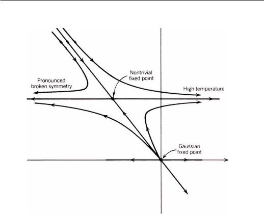
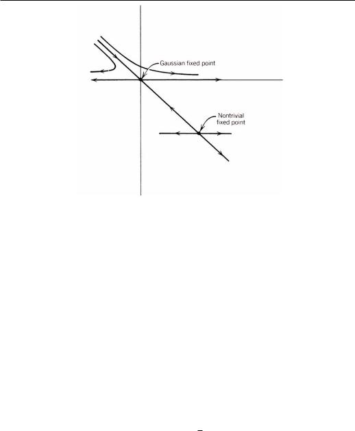
Now we have the following picture. For d < 4 ( > 0) the nontrivial fixed point lies in the upper half of the (x, y) plane whereas the Gaussian fixed point is at x = y = 0, see Fig.5.1. For the nontrivial fixed point, h2 is irrelevant (it does not affect the critical exponents) and h1 = r t the relevant scaling field whereas for the Gaussian fixed point, both field are relevant. Thus, the line ν2 is the critical line. For d > 4 ( < 0)the nontrivial fixed point lies in the
lower half of the (x, y) plane, i.e., in the unphysical region (u < 0), see |
Fig.5.2, |
and the critical behaviour is governed by the Gaussian fixed point. d |
= 4 is the |
special case when both fixed points coincide. The linearized recursion relations give x2 = 0, h2 is marginal, and x2 cannot tell us the direction of RG flow. In this case we must include higher–order terms which were neglected when we linearized the transformation matrix. These terms tell us that the scaling field h2 is irrelevant for u > 0 at d = 4.
Critical exponents
We have seen that the critical exponents of the nontrivial fixed point are
xt = 2 − /3
56
Phase transitions
A B C
y u
x r
Unphysical region
Figure 5.1: Fixed points and flow diagram of the Landau-Ginzburg-Wilson model for d < 4. The Gaussian fixed point at ( x , y ) = (0, 0) has the meanfield exponents. The non-trivial fixed point at ( x , y ) = (− /6, /36) is unstable against the relevant perturbation δx t and stable against the irrelevant perturbation δy. The system at A has t < 0 and it flows towards the low-temperature fixed point, r becomes increasingly negative. At the point C the system has t > 0 and it flows to the high-temperature fixed point, r becomes increasingly positive. The point B is on the critical line and the system flows towards the non-trivial fixed point.
57
Phase transitions
y u
x r
Unphysical region
Figure 5.2: Fixed points and flow diagram of the Landau-Ginzburg-Wilson model for d > 4. The nontrivial fixed point is in the unphysical region. To stabilize the system in the lower half of the (x, y) plane, one needs an m6 term.
xu |
= |
− |
(5.32) |
xh |
= |
1 + d/2. |
In fact, we calculated xh only for the Gaussian fixed point in the Eq. (5.12). However, the term with m4 does not affect the value of xh so that xh of the nontrivial fixed point is the same. With these values of x i we get
α |
= |
|
|
|
6 |
|
|
||
|
|
|
|
|
β |
= |
1 |
− |
|
|
|
|||
2 |
6 |
γ= 1 + 6
δ= 3 +
ν |
= |
|
1 |
|
+ |
|
|
|
2 |
|
12 |
||||||
|
|
|
|
|||||
η |
= |
0. |
|
(5.33) |
||||
58

Phase transitions
For d ≥ 4 ( ≤ 0) we only have the Gaussian fixed point in the physical region (u > 0) with the exponents
xt |
= |
2 |
|
xu |
= |
(5.34) |
|
xh |
= |
1 + d/2. |
|
Then we find
α |
= |
2 − |
d |
||||||
|
|
|
|
||||||
2 |
|
|
|||||||
|
|
1 |
|
− |
|
|
|||
(β |
= |
|
|
|
|
|
) |
||
2 |
|
4 |
|||||||
γ |
= |
1 |
|
|
|
|
|
|
|
(δ |
= 3 + ) |
||||||||
ν |
= |
|
1 |
|
|
|
|
|
|
2 |
|
|
|
|
|
|
|||
|
|
|
|
|
|
|
|
||
η |
= |
0. |
|
(5.35) |
|||||
The above expressions for β and δ are wrong, because we have neglected the m4 term in considering the Gaussian fixed point. Below TC , r is negative and for m to be finite the term um4 with u > 0 must be included in the Hamiltonian. Although u is an irrelevant field it helps to stabilize m at a finit value and in this way influence the critical behaviour. By treating the um4 term in the Gaussian approximation (independent modes) we get the usual mean-field values for the exponents β and η:
β |
= |
|
1 |
|
2 |
|
|||
|
|
|
||
δ |
= |
3 |
(5.36) |
|
for all d ≥ 4. These results are correct and also agree with the results of the Landau (MFA) model.
The Gaussian model gives the same critical exponents as the mean-field theory except for the specific-heat exponent α. Therefore the Gaussian fixed point is identified as the mean-field fixed point. In the Gaussian model the specific heat
59