

PHASE TRANSITION (lectures)
.pdfPhase transitions
0 |
|
|
|
|
|
|
|
|
|
|
|
|
|
0.5 |
|
|
|
-0.5 |
|
|
|
|
|
|
|
|
G(T,H) |
|
|
|
|
0.75 |
|
|
|
|
|
|
|
|
|
|
|
|
-1 |
|
|
|
|
1.0 |
|
|
|
|
|
|
|
|
T = 1.5 Tc |
|
|
|
-1.5 |
|
|
|
|
|
|
|
|
-2 |
|
|
|
|
|
|
|
|
-1 |
-0.75 |
-0.5 |
-0.25 |
0 |
0.25 |
0.5 |
0.75 |
1 |
|
|
|
|
H |
|
|
|
|
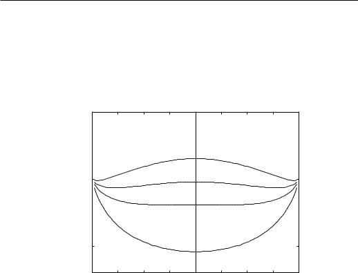
Figure 4.4: Equilibrium Gibbs free energy. At low temperatures, when a first order transition at H = 0 takes place, part of the curve corresponds to metastable states and part to unstable states.
of the variational parameter M0 above the critical temperature and a double minimum below TC. Close to the critical point and for H = 0, the minimum of G is close to m0 = 0 and we can expand the trial mean-field free energy G to a very good approximation in a power series of m.
G(T, H; m) = G0 + |
1 |
(4.23) |
2rm2 + um4 + · · · |
At T > TC, r must be > 0 and below TC, it must be < 0, thus r changes sign and in most of the cases it can be approximated by a linear temperature dependence,
r = r0(T − TC)/TC.
The Landau theory is phenomenological and deals only with macroscopic quantities. The theory does not deal correctly with the fluctuation and is a meanfield theory. In fact, the Landau theory of continuous phase transitions is much more than just simple expansion of G. It is based on the symmetry of the system. Landau postulated that the free energy can be expanded as a power series in m where only those terms that are compatible with the symmetry of the system are allowed.
40
Phase transitions
0 |
|
|
|
|
|
|
|
|
|
|
|
|
|
0.5 |
|
|
|
-0.5 |
|
|
|
|
0.75 |
|
|
|
|
|
|
|
|
|
|
|
|
F(T,m) |
|
|
|
|
|
|
|
|
|
|
|
|
|
1.0 |
|
|
|
-1 |
|
|
|
|
|
|
|
|
|
|
|
|
|
T = 1.5 Tc |
|
|
|
-1 |
-0.75 |
-0.5 |
-0.25 |
0 |
0.25 |
0.5 |
0.75 |
1 |
|
|
|
|
m |
|
|
|
|
Figure 4.5: Equilibrium Helmholtz free energy. At low temperatures, where the transition is first order, F has two minima, corresponding to ±m. The region between the two minima is the coexistence region when the system can be partially in the +m, and partially in the −m state (domain structure).
41

Phase transitions
Formulation of the Landau theory
Critical anomalies take place on long lenthscales. Therefore it is enough and in order to change from discrete to continuous description:
mi → m(~r) hi → h(~r).
In formulating the Landau theory let us consider a macroscopic system and assume that there exists a (generalized; not necessarily magnetic) order parameter density m(~r) averaged over microscopic, atomic distances a. Because of the average, m(~r) is now a continuous function of ~r (continuous in m and in ~r). There can be no fluctuation in m(~r) on the lengthscale smaller than a (a> lattice spacing). Correspondingly, m(~r) has no Fourier components with wavevector greater than
k = 2π/a.
In lattice models, the canonical partition function appropriate to the Gibbs free energy of a spin system is:
Y (T, H) = e−βH |
(4.24) |
{Xi} |
|
S |
|
(we have to sum over all spin configurations) Now, since m(r) is a continuous function of the coordinate r, we must replace the sum by a functional integral over all functions m(r). When doing this replacement one must not forget that m(r) is equal to the average of a microscopic spin Si over a small volume. That means that there can be several microscopic spin configuration which average into the same m(r). Let there be Ω(m(r)) spin configuration that lead to the same m(r). Then, the sum over all spin configuration is equal to the functional integral over all functions m(r) where each function m(r) is weighted by Ω(m(r)):
Si |
→ Z |
Dm(r) Ω(m(r)). |
(4.25) |
||
{X} |
|
|
|
|
|
The partition function is: |
|
|
|
|
|
Y (T, H) = Z |
Dm(r) Ω(m(r)) e−βH(H;m(r)). |
(4.26) |
|||
Using the Boltzmann formula S = kB ln Ω, we can write Y in the form: |
|
||||
Y (T, H) = |
Z |
Dm(r) e−βH(H;m(r)−T S) |
|
||
42

Phase transitions
Z
= Dm(r) e−βG(T,H;m(r)), (4.27)
where we have introduced the Landau free energy:
G(T, H; m(r)) = H(H; m(r) − T S(m(r)). |
(4.28) |
|
|
|
|
Notice the analogy between this equation and the trial Gibbs free energy obtained previously with the Bragg-Williams method. The Landau free energy is in fact a generalization of the trial Gibbs free energy.
Notice also that the entropy S(m(r)) is not equal to the usual microcanonical entropy S (related to the number of configuration in an energy interval E) because we did not make any summation over the energies. S (m(r)) is related to the number of microscopic configuration leading to the same function m(r). Only after integration over all the states in a certain energy interval we would get the usual thermodynamic entropy S. Therefore we can call S(m(r)) a partial entropy.
We still have to work out the functional integral in order to get the (equilibrium) partition function Y (T, H). From Y (T, H) the Gibbs free energy is:
Z
G(T, H) = −kBT ln Y (T, H) = −kBT ln Dm e−βG(T,H;m). (4.29)
In the Landau approach we write down the Landau free energy in a most general form as an expansion in terms of the order parameter and its derivatives by taking into account all the symmetry-allowed terms up to a given order:
|
Z |
dV |
1 |
|
|
|
|
G(T, H, m) = |
|
rm2 + um4 + · · · − Hm |
|
||||
2 |
|
||||||
|
|
|
+ |
1 |
g|rm|2 + · · · . |
(4.30) |
|
|
|
|
|
||||
|
|
|
2 |
||||
The highest-order coefficient in the expansion must always be positive, else the system were unstable. For the Ising model, this form can also be obtained by expanding G, Eq. (4.14), in powers of m. The last term appears if m is sitedependent:
SiSj → m(r) m(r + a) = m(r) m(r) + m(r) arm(r) + 12a2r2m(r) + · · · .
(4.31)
43

Phase transitions
The first term is already included in the first line of (4.30), the second term vanishes in systems with center of inversion (symmetry argument) and the last term, after partial integration over the whole volume, gives the term proportional to |rm|2. The prefactor g must also be positive always. A negative g would lead to completely unphysical wild fluctuation in m on extremely short lengthscales.
Here we have assumed a one-component order parameter. In general, the order parameter can have several components or be complex. The coefficient are in principle temperature-dependent and depend also on the symmetry of the system. For example, the coefficient of the cubic term vanishes if the system is invariant under the reversal of m(r) when H = 0. Usually we assume that u is temperature independent whereas the quadratic term has a linear temperature dependence,
r = r0t, |
t = (T − TC)/TC |
(4.32) |
In the Landau theory we assume that the fluctuation of the order parameter are small, that the important values of m lie in a narrow range near its equilibrium value that minimizes the Landau free energy. In fact, the maximal contribution to the partition function comes from the term with minimal Landau free energy. In the thermodynamic limit, the probability of any other configuration will vanish rapidly. Therefore we make use of the saddle-point approximation, the functional integral (4.29) is equal to the maximum value of the integrand, multiplied by a constant. For constant fiel H, the functional form of m(r) that maximizes the integrand (minimizes the Landau free energy), is a constant, determined by the conditions
∂G |
= 0 |
∂2G |
≥ |
0 |
(4.33) |
|
∂m |
∂m2 |
|||||
|
|
In the saddle-point approximation we immediately obtain G(T, H) from Eq. (4.29):
G(T, H) = G0 + minmG(T, H; m) = |
(4.34) |
In equilibrium, the system is at the bottom of the Landau free energy G. This determines m and G(T, H). From G(T, H) we get other thermodynamic quantities, as before.
The advantage of the Landau theory is that it allows one to study a macroscopic system without knowing all its microscopic details. It is based on the symmetry properties of the macroscopic system alone.
44

Phase transitions
Critical exponents in the Landau theory
We will now calculate the critical exponents of the Landau model. To be more specific let us investigate the Landau model of magnetic phase transitions, when
|
|
|
1 |
|
|
|
||
G |
= G0 + |
|
rm02 + um04 − m0H |
V |
(4.35) |
|||
2 |
||||||||
In equilibrium, when |
∂ |
G |
/∂m0 = 0 |
, we get the equation of state: |
|
|||
|
|
|
|
(4.36) |
||||
|
|
|
rm + 4um3 − H = 0 |
|
||||
Order-parameter exponent β ( H = 0). For H = 0, and r > 0, the equation of state has a single solution, m = 0, there is no spontaneous magnetization above TC, as expected. For t < 0, the equation of state has three roots when H = 0. The root at m = 0 belongs to an unstable state, so we are left with two real roots. The result is:
m2 = |
− |
r |
( |
m = |
s |
|
r0 |
|
t1/2 |
β = |
1 |
t < 0 |
(4.37) |
||
|
|
|
|
|
|||||||||||
4u |
2 |
||||||||||||||
4u |
|||||||||||||||
|
m = |
± |
|
|
t > 0 |
|
|||||||||
|
|
|
|
0 |
|
|
|
|
|
|
|
|
|||
Critical isotherm exponent δ (T = TC). Now, r = 0, and we have 4um3 = H, from which it follows
m = s3 |
|
H |
|
|
δ = 3 t = 0 |
(4.38) |
|||||||
|
4u |
||||||||||||
|
|
|
|
|
|
|
|
|
|
||||
Susceptibility exponent γ. The isothermal susceptibility is define |
as |
||||||||||||
|
|
|
|
|
|
|
|
∂m |
|
|
|
||
|
|
|
|
|
|
|
χT = |
|
|
! . |
|
|
(4.39) |
|
|
|
|
|
|
|
∂H |
|
|
|
|||
|
|
|
|
|
|
|
|
|
|
T |
|
|
|
From the equation of state, Eq. (4.36), we get: |
|
|
|||||||||||
|
|
|
! |
|
|
|
! |
|
|
|
|||
r |
∂m |
|
|
|
|
+ 12um2 |
∂m |
|
− 1 = 0 |
(4.40) |
|||
∂H |
|
|
T |
∂H |
T |
||||||||
|
|
|
|
|
|
|
|
|
|
|
|||
from which we find |
|
|
|
|
|
|
|
|
|
|
|
||
χT = ( |
1 |
|
|
t−1 |
|
γ = 1 t > 0 |
|
||||||
|
|
|
|
|
|
||||||||
|
r t |
|
|
|
|
||||||||
0 1 |
|
|t|−1 |
|
γ = 1 t < 0 |
(4.41) |
||||||||
|
|
|
|
|
|
||||||||
|
|
−2r0t |
|
|
|||||||||
45

Phase transitions
Specific-heat exponent α (H = 0). The specific heat at constant (zero) field is
cH = −T |
∂2G |
! |
(4.42) |
∂T 2 |
|||
|
|
|
H |
For t > 0, m = 0, and G = G0 = const. (that means that G0 does not depend on the reduced temperature t), so cH is zero. For t < 0 (and H = 0), m2 = −r/4u and
|
|
|
|
r02 |
(4.43) |
||
|
|
G = G0 − |
|
t2 |
|||
|
16u |
||||||
It follows: |
|
|
|
|
|
|
|
cH = ( |
0 |
|
α = 0 |
t > 0 |
|||
r02TC |
|
|
(4.44) |
||||
|
|
|
α = 0 |
t < 0 |
|||
|
|
8u |
|||||
Comment 1: We see that the Landau theory gives mean-field (also called ”classical”) critical exponents.
Comment 2: At H 6= ,0there is no phase transition, all the quantities vary smoothly, only the exponent δ is defined
Short-range order and fluctuations
Although the correlations and fluctuation are neglected in the MFA, we can still get an estimate of the short-range correlations. To obtain the mean-field values of the exponents ν and η, which describe the behaviour of the correlation function, we have to include the gradient term in the Landau free energy. In the framework of the mean-field theory, this leads to the Ornstein-Zernike approximation. To investigate the correlations, we consider the response of m(~r) to a perturbing field acting, say, at the origin, H(~r) = λδ(~r) via the “response function”, the susceptibility:
Z
m(~r) = ddr0χ(~r − ~r0)H(~r0). (4.45)
The Fourier transform of the last equation is simply:
m(~q) = χ(~q)H(~q). |
(4.46) |
46

Phase transitions
To the lowest order in m and rm, the Landau free energy is: |
|
||||||||
G(H; m(r)) = G0 + Z ddr |
1 |
|
1 |
|
|||||
|
g|rm(~r)|2 + |
|
|
rm2(~r) |
|
||||
2 |
2 |
|
|||||||
|
|
|
|
+um4(~r) − λm(~r)δ(~r)i |
(4.47) |
||||
We first make Fourier transforms to the d−dimensional momentum space, |
|
||||||||
m(~q) = Z |
ddr e−i~q·~rm(~r) |
|
|
|
|
||||
1 |
|
Z |
ddq ei~q·~rm(~q) |
|
|
|
(4.48) |
||
m(~r) = |
|
|
|
|
|
||||
(2π)d |
|
|
|
||||||
The Fourier transform of rm is:
rm(~r) = |
1 |
Z |
ddq |
rei~q·~r m(~q) |
(2π)d |
||||
= |
1 |
Z |
ddq i~qei~q·~rm(~q) |
|
|
||||
(2π)d |
||||
The Fourier transform of a δ−function is a constant,
δ(~r) = |
1 |
Z |
ddq ei~q·~r |
(2π)d |
In the momentum space, the Landau free energy is:
G(H; m(~q)) = G0 + Z ddq 12gq2m2(~q) + 12rm2(~q)
i
+um4(~q) − λm(~q) .
(4.49)
(4.50)
(4.51)
Here, we approximated the Fourier transform of m4(~r) by m4(~q)!
In the mean-field approximation the modes with different momenta ~q are assumed to be independent of each other. Therefore we can minimize G for each individual mode separately,
∂G |
= 0, |
(4.52) |
|
∂m(~q) |
|||
|
|
and the equation of state in momentum space is:
(gq2 + r)m(~q) + 4um3(~q) = λ. |
(4.53) |
47

Phase transitions
For t > 0, when m vanishes in the absence of the field we can neglect the cubic term, and we get:
|
λ |
|
1 |
|
|
m(~q) = |
|
, |
χ(~q) = |
|
. |
gq2 + r |
gq2 + r |
||||
After a Fourier transform back to real space we find in the limit of large ~r:
χ(~r) m(~r) r2−d exp(−r/ξ) η = 0
where |
|
|
|
|
|
|||
|
|
|
|
|
|
1 |
||
ξ = r |
g |
|
|
|||||
|
|
ν = |
|
|
. |
|||
r0t |
2 |
|||||||
(4.54)
(4.55)
(4.56)
Below TC, m 6= 0, we replace m(~r) by m+δm(~r), where m is the spontaneous
magnetization and δm the response to the infinitesimal perturbing field |
λ. We |
||
expand in powers of δm and retain only linear-order terms. We find |
|
||
δm(~q) = |
λ |
(4.57) |
|
|
|
||
gq2 − 2r |
|||
and the same exponents as for t > 0.
In the Ornstein-Zernike approximation (random-phase approximation), the modes with different momenta are considered to be independent of one another. The free energy is a sum (integral) of contributions from non-interacting normal modes.
Validity of the mean-field theory
The mean-field theories neglect the fluctuation of the neighbouring spins, each spin interacts only with the mean value of its neighbours. So, the mean-filed theories can only be valid when fluctuation are irrelevant. We will now estimate the relevance of fluctuation close to the critical point. We shall calculate the free energy of the fluctuation and compare it with the free energy calculated in the MFA.
To the order of magnitude, only those fluctuation can be thermally excited whose free energy is of the order kBT (or less). The free energy of a typical fluctuation will thus be proportional to kBT . Since the size of the fluctuation is of
48

Phase transitions
the order of the correlation length ξ (this is how the correlation length is defined) the free energy of a typical fluctuation per unit volume is proportional to
Gfluct ξ−d |t|νd. |
(4.58) |
On the other hand, the singular part of the mean-field |
free energy is governed by |
the specific-heat exponent α: |
|
GMF |t|2−α
(we obtain this expression after two integrations of the specific ature). For the mean-field theory to be ”exact”, Gfluct
t → 0,
lim |
|
Gfluct |
|
lim |
t νd−2+α = 0 |
||||||
|
GMF |
||||||||||
|t|→0 |
|
|t|→0 |
| | |
2 − α |
|
||||||
|
νd |
− |
2 + α > 0 |
|
d > |
. |
|||||
|
|
|
|
|
ν |
||||||
For the Ising model (scalar order parameter) in the mean-field 0 and ν = 1/2 and we get the condition
(4.59)
heat over temperin the limit as
(4.60)
approximation α =
d > 4. |
(4.61) |
The mean-field exponents are correct and the fluctuation |
are irrelevant only for |
d > 4. d = 4 is called the upper critical dimension of the Ising model.
49