PHASE TRANSITION (lectures)

Phase transitions

from which we find

If we insert this expression into the equation of state, Eq. (3.17), we obtain the pressure at which the transition takes place:

At TC , the ensemble average of the density of particles in the continuum states reaches its maximum value whereas the ground state is still empty, hN0i/V = 0.

Below TC , hNmax0 i further decreases and becomes < N (we keep N fixed). The chemical potential further approaches zero (µ cannot be exactly = 0, because that would mean that N = ∞) and z → 1 in such a way that the total number of particles is kept constant. z is very close to 1, we can put gn(z) ≈ gn(1) and the number of particles in the continuum states is

When hN0i < N, the ground state starts to fill hN0i increases. Below TC , thus, only a part of the particles can be accommodated in the continuum states. The rest must go into the ground state! The number of bosons in the ground state is:

from which we get:

hN0i/N is finite the state with p~ = 0 is occupied with a macroscopic number of particles, the particles condense in the momentum space into the zero-momentum

30

Phase transitions

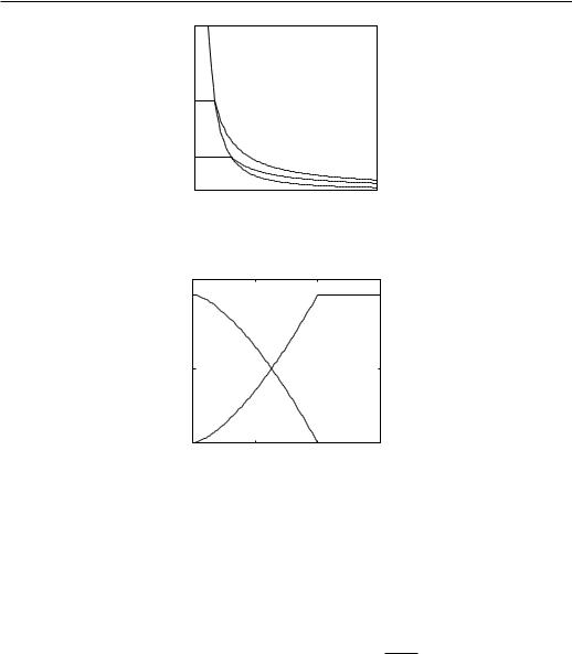
Figure 3.2: Isotherms of the ideal Bose gas.

Figure 3.3: Temperature dependence of the relative number of bosons in the ground (hN0i/N) and excited (hN0i/N) states.

state. This is the Bose-Einstein condensation. The fugacity is, from Eq. (3.13): z = hN0i/(hN0i + 1). In the thermodynamic limit, when V and hN0i → ∞, z = 1 and µ = 0 below TC . The equation of state is:

Only the particles in the continuum states (in the gas phase) contribute to pressure. The particles in the ground state (condensate) are at rest, they cannot exert any pressure. If the density is increased, the extra particles fall into the ground state and the pressure does not increase. At fixed T < TC the density of particles in the gas phase is constant and P is independent of V , see Fig. 3.2. The temper-

ature dependence of hN0i is shown in Fig. 3.3. In the limit T → 0, hNmax0 i → 0 and all the particles are in the ground state, N = hN0i.

31

Phase transitions

P

Vacuum

Gas phase

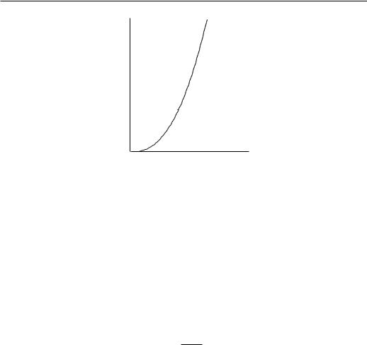
Figure 3.4: Phase diagram of an ideal Bose gas.

The corresponding phase diagram is shown in Fig. 3.4. The normal, gas phase exists for T > TC , i.e., to the right of the transition line. On the line, given by (3.24), condensation takes place and since the particles in the ground state don’t contribute to pressure, the condensate lies on the transition line itself. Notice that the ”critical points” in Bose systems form a line in the P vs. T or in the P vs. V planes and are not in a single point like in van der Waals gases.

We now invert Eq. (3.27),

condensed phase does not occupy any volume. This means that the ideal Bose gas can be compressed to zero volume without any increase in pressure.

Some comments: The condensate (ground state) contributes neither to E, nor to CV , P , or V . At low T , CV vanishes like T 3/2 in contrast to the photon gas, where CV T 3. They differ because the density of states is different in both cases. There are more excited states available for particles than for photons and the specific heat is greater.

Of course, this, and infinit compressibility are the artifacts of the ideal gas model. In reality, because of atomic repulsion, the volume of the condensed phase does not vanish and the compressibility does not diverge.

32

Phase transitions

Mean-field theories

Very few models of statistical mechanics have been solved exactly; in most of the cases one has to rely on approximative methods. Among them, the mean-field approximation (MFA) is one of the most widely used. The advantage of the meanfield theory is its simplicity and that it correctly predicts the qualitative features of a system in most cases.

The essence of the mean-fiel theory is the assumption of statistical independence of the local ordering (spins in the case of magnetic systems). The interaction terms in the Hamiltonian are replaced by an effective, ”mean field term. In this way, all the information on correlations in the fluctuation is lost. Therefore, the mean-field theory is usually inadequate in the critical regime. It usually gives wrong critical exponents, in particular at low spatial dimensions when the number of NN is small.

The MFA becomes exact in the limit as the number of interacting neighbours z → ∞. This is the case when the range of interaction z → ∞ or if the spatial dimension is high. In both cases, a site ”feels” contributions from many neighbours and therefore the fluctuation average out or become even irrelevant (for Ising systems, they become irrelevant in d ≥ 4). At low d, the MFA must be used with caution. Not only that it predicts wrong critical exponents, its predictions are even qualitatively wrong sometimes. For example, it predicts long-range order and finit critical temperature for the d = 1 Ising model. In the following, we shall introduce and formulate the MFA for magnetic system. The results

33

Phase transitions

however, are valid also for other systems.

Two formulations of the mean-field approximation. We will now formulate the mean-field approximation in two different ways.

•A: The “Weiss molecular field theory” according to its “inventor” Pierre Weiss. This method is straightforward and easy to understand. It gives us an expression for the order parameter but does not tell us anything about the free energy or partition function.

•B: The second method will be the Bragg-Williams approximation which is more sophisticated and is based on the free energy minimization.

We will develop the mean-field approximation on the Ising model in an external magnetic field

Weiss molecular field of an Ising system

Weiss formulated a theory of ferromagnetism in which he assumed that the effect of the neighbouring spins on a given spin can be described by a fictitious molecular field which is proportional to the average magnetization of the system.

We start with the Ising Hamiltonian in an external magnetic field

It depends on the configuration of all the neighbouring spins around the site i. If the lattice is such that each spin has many neighbours, then it is not a bad approximation to replace the actual value of the neighbouring spins by the mean value of all spins,

X Sj → zm, (4.3)

j

where z is the number of nearest neighbours and m is the mean (average) magnetization per site, m = N1 Pj Sj. With (4.3), the local field becomes

34

Phase transitions

1.0

T/Tc

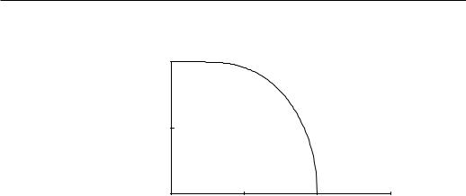
Figure 4.1: Temperature dependence of the order parameter in the mean-field approximation.

The actual local field acting on the site i was replaced by its mean value and is independent of the site, Hi → HMF . In the mean-fiel approximation the original Hamiltonian is replaced by a mean-field Hamiltonian

HMF = −HMF X Si, (4.5)

i

which is equivalent to the Hamiltonian of a non-interacting spin system in an external magnetic field and can be solved exactly:

This is a self-consistent, transcendental equation for m. It has a non-trivial solution (m 6= 0) forβzJ > 1, i.e., at low temperatures. The temperature dependence of the order parameter m for H = 0 is shown in Fig. 4.1. It vanishes at the critical temperature TC = zJ.

Bragg-Williams approximation

The Gibbs free energy is a function of T and H,

35

Phase transitions

This equation tells us that for fixed T and H, δG = 0. In equilibrium, thus, G is an extremum of a trial free energy G with respect to any variational parameter. We will now search the trial free energy G.

We start with the density matrix and calculate the Gibbs free energy of an Ising system. In the Bragg-Williams (mean-field approach we approximate the total density matrix ρ by a direct product of the density matrices for individual spins,

Physically this means that the spin fluctuation are considered to be uncorrelated, the orientation of a spin is statistically independent of the orientation of any other spin. There are no correlations in the spin orientation except those coming from the long-range order. Under this assumption, the Ising Hamiltonian is not only diagonal in the spin space (the state Si = +1 is uncoupled from the state Si = −1; physically this means that the Ising system has no dynamics), but it is also independent of all other spins in the system. Thus, the trial density matrices ρi are diagonal and of the general form (remember, its trace must be = 1):

They depend on the variational parameter which is site-independent, m0i = m0, because of translational invariance. With this density matrix the average spin orientation is:

Because of statistical independence of the spins in MFA, the short-range spin correlations are:

We can write the (trial) enthalpy E = hHi [where H is given by the Eq. (4.1)] as:

36

Phase transitions

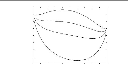
Figure 4.2: Trial Gibbs free energy G(T, H; m0) vs. m0 at H = 0.1 zJ. Solid circles denote stable states, open circle a metastable state, and the solid triangle an unstable state. The curves are labelled by T/TC. m and G(T, H) are determined by the minimum of G.

It depends on H, T , and on the variational parameter m0. G for H = 0.1 (in units of zJ) is shown in Fig. 4.2. To get the true equilibrium Gibbs free energy, G(H, T ; m) has to be minimized with respect to the variational parameter m0,

The minimization gives:

37

Phase transitions

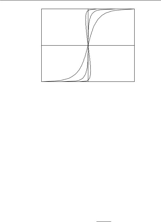
Figure 4.3: External-field dependence of the Ising-model magnetization in the mean-field approximation. TC is the critical temperature. Solid line: stable states, dashed line: metastable states, dotted line: unstable states.

or:

This is the familiar “equation of state” of magnetic systems.

The field-dependence of m, Eq. (4.17) is shown in Fig. 4.3. At high temperatures (T > TC), the order parameter m behaves as in a paramagnet, this is the paramagnetic phase. The spins are partially ordered only because of H. For H = 0, the spins are disordered, therefore this phase is also called the disordered phase. At low temperature (T < TC), the spins are spontaneously ordered even in the absence of H. This is the spontaneously ordered phase. The system has long-range order for J > 0, all the spins are oriented predominantly in the same direction, this is the ferromagnetic phase.

The Gibbs free energy is:

38

Phase transitions

where m is related to H via the Eq. (4.17). The equation of state is

T

The Helmholtz free energy is F (T, M) = G(T, H) + HM:

The field dependence of the equilibrium Gibbs free energy G is shown in Fig. 4.4. The equation of state now reads

The Helmholtz free energy F (T, M, N) is shown in Fig. 4.5.

As before, the critical temperature, where the spontaneous ordering vanishes in the absence of external magnetic field H as T is increased, is determined by the condition βCzJ = 1,

In the past, many improvements to the simple MF theory presented here have been proposed. With these improvements, the MF critical temperature came closer to the exact critical temperature. None of these theories, however, was able to bring an improvements to the critical exponents, they kept their mean-field values. The real break-through brought the renormalization-group theory, which will be introduced latter.

Landau theory of continuous phase transitions

In the previous section we have seen that the trial Gibbs free energy G (T, H; M0) was an analytic function which had approximately a parabolic shape as a function

39