

PHASE TRANSITION (lectures)
.pdfPhase transitions
arranged on a ring, see Fig. 2.3. Then, the N−th and the first spins are NN and the system is periodic. The partition function is:
Z = S |
e−βH({S}) = |
S |
eβJ Pi SiSi+1 = |
S |
N |
(2.24) |
i=1 eβJSiSi+1 . |
||||||
X{ } |
|
X{ } |
|
X{ } |
Y |
|
(Don’t forget: P{S} is the sum over all spin configu ations – there are 2N spin configuration – whereas Pi is the sum over all sites!)
The exponent in (2.24) can be written as:
eβJSiSi+1 = cosh βJSiSi+1+sinh βJSiSi+1 = cosh βJ+SiSi+1 sinh βJ. (2.25)
The last equality holds because SiSi+1 can only be ±1 and cosh is an even function whereas sinh is an odd function of the argument. The partition function is:
|
X{ } |
N |
(2.26) |
Z = (cosh βJ)N |
[1 + KSiSi+1] , |
||
|
Y |
|
|
|
S |
i=1 |
|
where K = tanh βJ. We work out the product and sort terms in powers of K:
Z = (cosh βJ)N X(1 + S1S2K)(1 + S2S3K) · · · (1 + SN S1K)
{S}
= (cosh βJ)N X [1 + K(S1S2 + S2S3 + · · · + SN S1)+
{S}
+K2(S1S2S2S3 + · · ·) + · ·· + KN (S1S2S2 · · · SN SN S1)i . (2.27)
The terms, linear in K contain products of two different (neighbouring) spins, like SiSi+1. The sum over all spin configuration of this product vanish, P{S} SiSi+1 = 0, because there are two configuration with parallel spins (SiSi+1 = +1) and two with antiparallel spins (SiSi+1 = −1). Thus, the term linear in K vanishes after summation over all spin configurations. For the same reason also the sum over all spin configurations which appear at the term proportional to K2, vanish. In order for a term to be different from zero, all the spins in the product must appear twice
(then, |
{Si} |
S2 = 2). This condition is fulfille only in the last term, which – af- |
||
|
|
i |
|
|
ter |
summation over all spin configuration – gives 2N KN . Therefore the partition |
|||
|
P |
|
|
|
function of the Ising model of a linear chain of N spins is: |
|
|||
|
|
|
Z = (2 cosh βJ)N h1 + KN i . |
(2.28) |
20
Phase transitions
In the thermodynamic limit, N → ∞, KN → 0, and the partition function becomes:
Z(H = 0) = (2 cosh βJ)N . |
(2.29) |
|
|
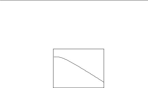
The free energy,
0 |
F/N |
Temperature |
Figure 2.4: Free energy of the Ising model in d = 1.
F = −NkBT ln(2 cosh βJ), |
(2.30) |
is regular at all finit T , therefore the Ising model in d = 1 has no phase transition at any finit T .
To investigate the possibility of a phase transition at T = 0, we will calculate
the correlation function and the correlation length ξ. We first |
replace J by Jj |
|
(at the end we put Jj = J), so that |
|
|
Z = 2N Yj |
cosh βJj. |
(2.31) |
The nearest-neighbour spin-spin correlation function is:
(i, i + 1) = |
hSiSi+1i = |
1 |
|
SiSi+1eβ Pj |
JjSjSj+1 |
||||
|
|
||||||||
Z S |
|
||||||||
|
|
1 |
|
∂Z |
|
|
X{ } |
|
|
= |
|
|
= tanh (βJi). |
(2.32) |
|||||
|
|
|
|||||||
|
βZ ∂Ji |
|
|
|
|
||||
The spin correlation function for arbitrary distance k,
(i, i + k) = hSiSi+ki
21
Phase transitions
= hSiSi+1Si+1Si+2Si+2Si+k−1Si+k−1Si+ki |
|
||||||||||
|
1 ∂ |
|
∂ |
|
∂ |
∂ |
(2.33) |
||||
= |
|
|
|
|
|
|
|
· · · |
|
Z, |
|
Z |
∂(βJi) |
∂(βJi+1) |
∂(βJi+2) |
∂(βJi+k−1) |
|||||||
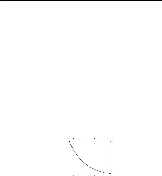
(k) ≡ (i, i + k) = [tanh (βJ)]k, |
|
|
(2.34) |
||||||||
is just the product of all the nearest-neighbour correlation functions between the sites i and i+ k, and is (if all J’s are equal) independent of the site i. The decay of the spin correlation function with distance is shown in Fig. 2.5. The correlations decay exponentially with distance and the correlation length is:
|
ξ |
1 |
|
(2.35) |
||
|
|
|
= − |
|
, |
|
a |
ln tanh βJ |
|||||
|
|
|
|
|
|
|
where a is the separation between the NN spins (”lattice constant”). In the limit T → 0, the correlation length diverges exponentially as T → 0:
|
ξ |
≈ |
1 |
e2βJ . |
(2.36) |
|
|
|
|
|
|||
|
a |
2 |
||||
Equations 2.34 and 2.36 tell us that there is no long range order at any finit |
T and |
|||||
1 |
|
|
|
|
|
Γ |
|
|
|
|
|
0 |
|
|
|
|
|
0 |
2 |
4 |
6 |
8 |
10 |
|
|
|
k |
|
|
Figure 2.5: Decay of the correlations in the d = 1 Ising model.
that T = 0 is the critical temperature of the d = 1 Ising model. Such a behaviour is typical for systems in the lower critical dimension:
d > dC : |
TC 6= 0 |
(2.37) |
d ≤ dC : |
TC = 0, |
(2.38) |
22

Phase transitions
therefore we conclude that d = 1 is the lower critical dimension of the Ising model.
The zero-fiel isothermal susceptibility of the d = 1 Ising model is, according to the fluctuation-dissipation theorem,
β X
χT (H = 0) = N i,j hSiSji.
In the thermodynamic limit, χT becomes:
|
β |
|
|
N/2 |
|
|
|
|
|
|
X k=X− |
|
|
|
|
|
|||
|
|
|
|
|
|
|
|||
|
|
|
|
|
|
|
|||
χT (H = 0) = N i |
|
N/2hSiSi+ki |
|
|
. |
||||
= |
β |
|
2 N/2 |
SiSi+k |
|
SiSi |
|
||
|
|
X |
|
X |
|
i − h |
|
i |
|
|
N i |
|
k=0h |
|
|
|
|||
In the thermodynamic limit (N → ∞), χT (H = 0) becomes
"#
|
2 |
− 1 |
1 |
e2J/kBT . |
|
χT (H = 0) = β |
|
= |
|
||
1 − tanh βJ |
kBT |
||||
(2.39)
(2.40)
(2.41)
The susceptibility has an essential singularity of the type exp(1/T ) as T → TC = 0 when J > 0. When J < 0, i.e., for antiferromagnetic NN interaction, the spin correlation function alternates in sign and the susceptibility is finit at all T .
The internal energy is:
E = −∂ ln Z/∂β = −JN tanh βJ. |
(2.42) |
Notice the similarity between the internal energy and the short-range correlation function (i, i + 1)! This is a general property of the internal energy.
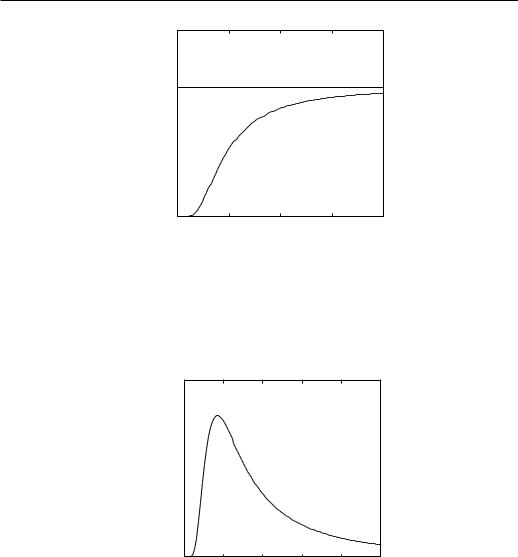
The entropy is S = (E − F )/T ,
S(H = 0) = NkB ln [2 cosh βJ] − |
NJ |
|
|
T |
In the limit T → 0, S → 0 and in the limit T → ∞, S The heat capacity CH = T (∂S/∂T )H is:
tanh βJ. |
(2.43) |
→ NkB ln 2, see Fig. 2.6.
βJ |
2 |
|
|
! . |
(2.44) |
||
CH = NkB cosh βJ |
The heat capacity is finit at all temperatures (no singularity at T = 0), see Fig. 2.7.
23
Phase transitions
|
|
N k ln(2) |
|
|
S |
|
|
|
|
0 |
1 |
2 |
3 |
4 |
|
|
kT/J |
|
|
Figure 2.6: Temperature dependence of the entropy for the zero-field d = 1 Ising model.
CH |
|
|
|
|
|
0 |
1 |
2 |
3 |
4 |
5 |
|
|
kT/J |
|
|
|
Figure 2.7: Temperature dependence of the heat capacity for the zero-field d = 1 Ising model.
24

Phase transitions
Bose systems
Ideal Bose gas
Now we shall consider the properties of an ideal gas of particles with integer spin and mass m > 0. As usually for ideal gases, we neglect the interaction between the particles. The Hamiltonian of the ideal Bose gas is:
X p2
H = p~ 2m np~.
np~ is the number of particles in the state with momentum p~. Because we are dealing with Bosons, np~ can also be > 1. We want to study condensation where two phases come into contact, the number of particles in one phase is not fixed, therefore we must work with the grand-canonical distribution. The grand-canonical partition function of ideal Bose gas is:
Ξ = np~ |
e−β Pp~ (p2/2m) np~+βµN , |
N = p~ |
np~. |
{X} |
|
X |
|
(Here we will disregard the (2S + 1) factor which comes from the spin degeneracy.) In the grand partition function, each sum over np~ is over all non-negative integers and, since the particles do not interact, we can split the partition function into a product:
∞ |
∞ |
· · · nheβµi |
n0 |
2 |
/2m−µ)i |
n1 |
2 |
/2m−µ)i |
n2 |
· · ·o = |
(3.1) |
Ξ = n0=0 |
n1=0 |
|
he−β(p1 |
|
he−β(p2 |
|
|||||
X X |
|
|
|
|
|
|
|
|
|
|
|
()
= |
p~ |
n |
2 |
/2m−µ)i |
n |
p~ |
1 |
|
1 |
/2m . |
|
he−β(p |
= |
|
ze−βp2 |
||||||||
|
Y X |
|
|
|
Y |
|
− |
|
|
|
|
Here we have introduced the fugacity z = eβµ. The equation of state of an ideal Bose gas is:
|
|
P V = kBT ln Ξ(T, V, µ) |
|
|||
|
|
|
|
|
|
|
|
P V |
= − |
p~ |
2 |
/2m−µ)i |
(3.2) |
kBT |
ln h1 − e−β(p |
|||||
|
|
|
X |
|
|
|
|
|
|
|
|
|
|
25

Phase transitions
The thermal average of N is determined by the chemical potential µ: |
|
|||||||||||||
1 |
∂ ln Ξ |
|
|
|
1 |
|
|
|
(3.3) |
|||||
hNi = − |
|
|
|
|
|
= |
p~ |
|
|
|
|
|
. |
|
β |
|
∂µ |
eβ(p2 |
/2m−µ) |
− |
1 |
||||||||
|
|
|
|
|
|
|
X |
|
|
|
|
|
||
We can write hNi = Pp~ np~ where |
|
1 |
|
|
|
|
|
|
(3.4) |
|||||
|
np~ = |
|
|
|
|
|
|
|
|
|
||||
|
|
|
|
|
|
|||||||||
|
eβ(p2/2m−µ) − 1 |
|
|
|
||||||||||
is the Bose-Einstein distribution function, which tells the occupation probability of a given (non-degenerate) state p~. For hNi to be finit and positive, the second term in the denominator has to be < 1 for any p~, in particular for p = 0. This means that µ must be < 0 and 0 < z < 1.
For large V we replace the sum by an integral: |
|
|||||||||||||||||||
|
p~ |
|
|
|
|
|
πV |
|
Z0∞ p2 dp |
|
|
|
(3.5) |
|||||||
|
→ 4h3 |
|
|
|
|
|||||||||||||||
|
X |
|
|
|
|
|
|
|
|
|
|
|
|
|
|
|
|
|
|
|
and we get: |
|
Z0∞ p2 dp eβ(p2/2m−µ) − 1 |
|
|||||||||||||||||
hNi = h3 |
|
|
||||||||||||||||||
|
4πV |
|
|
|
|
|
|
|
|
|
|
|
|
|
|
|
1 |
|
|
|
= V g3/2(z) |
|
|
mkBT |
! |
3/2 |
= |
V |
g3/2(z), |
(3.6) |
|||||||||||
|
|
|
|
|
|
|
|
|
||||||||||||
|
|
|
2πh¯2 |
|
|
|
λ3 |
|||||||||||||
where |
|
|
|
|
|
|
|
|
|
|
|
|
|
|
|
|
|
|
|
|
1 |
|
Z0∞ dx |
|
|
xν−1 |
|
|
∞ zl |
(3.7) |
|||||||||||
gν(z) = |
|
|
|
|
|
= l=1 |
|
|||||||||||||
(ν) |
exz−1 |
− |
1 |
lν |
||||||||||||||||
|
|
|
|
|
|
|
|
|
|
|
|
|
|
|
X |
|
||||
and λ is the thermal wavelength, |
|
|
|
|
|
|
|
|
|
|
|
|
|
|
|
|
||||
|
|
|
|
|
|
|
2πh¯2 |
|
|
1/2 |
|
|
|
|
|
|
||||
|
λ = |
|
|
! . |
|
|
|
|
|
|||||||||||
|
|
|
mkBT |
|
|
|
|
|
||||||||||||
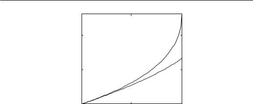
The functions g3/2(z) and g5/2(z) are shown in Fig 3.1. For later use: 2.612 and g5/2(1) ≈ 1.342. The pressure is:
P = |
m |
(kBT )5/3g5/2(z) = |
kBT |
g5/2(z). |
2πh¯2 |
λ3 |
g3/2(1) ≈
(3.8)
26
Phase transitions
2 |
|
3/2 |
|
|
|
g |
|
|
1 |
|
5/2 |
|
|
|
0 |
0.5 |
1 |
|
z |
|
Figure 3.1: The functions g3/2(z) and g5/2(z). |
||
Now let us start increasing the pressure at fixed (high enough) T . This increases the chemical potential, the fugacity, and the density of particles, hNi/V . However, we know that z must be < 1. What happens when z → 1? Can we further increase the pressure or the density of particles?
To answer this question we must go back to Eq. (3.3). The term with p~ = 0 which was not included in (3.6) (The density of states n(E) has a √E dependence on E and vanishes as E → 0.) becomes singular (divergent) when µ → 0 and it has to be treated separately. This divergence has very important consequences for a Bose gas, as we shall show now. Instead of Eq. (3.3) we must write:
1 |
|
|
|
|
z |
|
|
V |
|
|
z |
|
(3.9) |
||
hNi = p~ =0 |
|
|
|
+ |
|
|
|
= |
|
g3/2 |
(z) + |
|
|
|
|
eβ(p2/2m−µ) |
− |
1 |
1 |
− |
z |
λ3 |
1 |
− |
z |
||||||
X6 |
|
|
|
|
|
|
|
|
|
|
|
||||
and the equation of state is:
kBT |
= − |
4h3 |
|
Z0∞ p2 dp ln h1 − ze−βp |
/2mi |
− ln (1 − z) |
|
|||||||
P V |
|
|
πV |
|
|
|
|
|
|
2 |
|
|
|
|
|
|
|
|
|
|
|
|
|
|
|
|
|
|
|
|
|
|
P |
|
|
1 |
1 |
|
|
|
|
(3.10) |
||
|
|
|
|
|
= |
|
|
g5/2(z) − |
|
ln (1 − z) , |
|
|||
|
|
|
kBT |
|
λ3 |
V |
||||||||
|
|
|
|
|
|
|
|
|
|
|
|
|
|
|
27

Phase transitions
The last terms in Eqs. (3.9) and (3.10) come from the term p = 0 and correspond to the particles in the lowest energy, in the ground state. In the thermodynamic
limit the last term in (3.10) vanishes whereas it remains finit |
in (3.9). We will |
denote |
|
hNi = hN0i + hN0i, |
(3.11) |
where hN0i is the average number of bosons in the continuum (excited, p > 0) states,
hN0i = |
V |
g3/2(z) |
(3.12) |
λ3 |
and hN0i the average number of bosons in the ground state,
hN0i = |
z |
(3.13) |
1 − z . |
The average density of bosons in the continuum states reaches its maximum value when g3/2(z) is maximal, that is for z → 1 (µ → 0),
h |
N0 |
(T ) |
i = g3/2 |
(1) |
mkBT |
! |
3/2 |
(3.14) |
||
V |
|
|
2πh¯2 |
T 3/2. |
||||||
|
max |
|
|
|
|
|
|
|
|
|
The fact that hN0i is limited and cannot exceed hNmax0 i has its origin in the quantum-mechanical and statistical nature of the system. The number of avail-
able states in a box with volume V is finit and is equal to λV3 . Each state, on the average, accommodates np~ particles, where np~ is given by the Bose-Einstein distribution function, Eq. (3.4). If there are more than hN0 i particles in the system, they are pushed into the ground state.
Bose Einstein condensation
We will now investigate the behaviour of ideal Bose gases, described by Eqs. (3.9, 3.10). Let us consider a system of N bosons in a volume V .
At high enough temperature, hNmax0 i is so large that N < hNmax0 i and the chemical potential is determined from
N = hN0i = V |
mkBT |
! |
3/2 |
(3.15) |
|
g3/2(z). |
|||
2πh¯2 |
28

Phase transitions
This means that z < 1 and µ < 0. The density of particles in the ground state is
hN0i/V = z/(1 − z)/V → 0 as V → ∞. |
(3.16) |
Almost all the particles are in the |p~| > 0 states and the ground state is macroscopically empty. The equation of state simplified to
P |
= |
g5/2(z) |
|
(3.17) |
|
kBT |
λ3 |
||||
|
|
||||
At very high T , g3/2(z) and g5/2(z) are 1 and we approximate [see the series for gn, Eq. (3.7)]:
|
|
|
|
|
|
g5/2(z) ≈ g3/2 ≈ z |
|
|
|
|
|
|
|
|
|
(3.18) |
||||||||
and the equation of state becomes: |
|
|
|
|
|
|
|
|
|
|
|
|
|
|
|
|||||||||
|
|
P |
|
|
|
mkBT |
|
3/2 |
|
mkBT |
3/2 |
|
|
|
z |
|
||||||||
|
|
|
|
|
= g5/2(z) |
|
|
|
! |
≈ z |
|
|
|
|
! |
= |
|
|
|
. |
(3.19) |
|||
|
kBT |
|
|
2πh¯2 |
|
2πh¯2 |
|
|
λ3 |
|||||||||||||||
z is determined by the density of particles: |
|
|
|
|
|
|
|
|
|
|
|
|
|
|||||||||||
|
N |
|
|
mkBT |
3/2 |
mkBT |
|
|
3/2 |
|
|
z |
|
|||||||||||
|
|
|
|
= g3/2(z) |
|
! |
|
≈ z |
|
|
! |
= |
|
. |
(3.20) |
|||||||||
|
|
V |
2πh¯2 |
|
2πh¯2 |
λ3 |
||||||||||||||||||
The fugacity z = hNiλ3/V vanishes as T −3/2 at high T and for fixed density. This justifie the approximation (3.35). Eliminating z from the last two equations yields the equation of state of the ideal Bose gas at high T :
P V =< N > kBT |
(3.21) |
|
|
which is identical to the equation of state of a classical ideal gas (as it should be at high T).
Now we lower the temperature by keeping N and V fixed. Eq. (3.15) tells us that g3/2(z) must increase. This means that z and µ also increase. Eventually, a temperature is reached, where z reaches its maximum value (z → 1, N = hNmax0 i). This is the transition temperature TC and is determined by the condition
N |
|
mkBTC |
! |
3/2 |
|
= g3/2(1) |
(3.22) |
||||
V |
2πh¯2 |
29