PHASE TRANSITION (lectures)

Phase transitions

the Ising model in d = 2 forms one universality class, whereas in d = 3 it forms another universality class, the Ising models in d = 2 and d = 3 have different critical exponents because they have different spatial dimensionality. However, on a first glance very different physical systems often belong to the same universality class. Example: binary alloys and some magnetic systems can be described with mathematically similar models and they belong to the same universality class. Roughening of some crystal surfaces at high temperature (but below the melting temperature) and the d = 2 Coulomb gas are members of another universality class.

11

Phase transitions

Classical models

In this section we will discuss models that can be described by classical statistical mechanics. We will concentrate on the classical spin models which are used not only to study magnetism but are valid also for other systems like binary alloys or lattice gases.

In principle, all particles obey quantum statistical mechanics. Only when the temperature is so high and the density is so low that the average separation between the particles is much larger than the thermal wavelength λ,

the quantum statistical mechanics reduces to classical statistical mechanics and we can use a classical, Maxwell-Boltzmann distribution function (instead of Fermi– Dirac or Bose–Einstein).

For magnetic materials, the situation is somewhat different. The Hamiltonian of a magnetic system is a function of spin operators which can usually not be directly approximated by classical vectors. Quantum models in d dimensions can be mapped onto classical models in d0 = (d + 1) dimensions. The classical limit of the Heisenberg model, however, can be constructed for large eigenvalues of the spin operator by replacing the spin operators by three-dimensional classical vectors.

There is another quantum-mechanical effect we must discuss. In quantum mechanics identical particles are indistinguishable from each other whereas in classical mechanics they are distinguishable. Therefore, the partition function of a system of non-interacting, non-localized particles (ideal gas) is not just the product of single-particle partition functions, as one would expect from classical statistical

12

Phase transitions

mechanics, but we must take into account that the particles are indistinguishable. We must divide the total partition function by the number of permutations between N identical particles, N!,

where Z1 is the one-particle partition function. The factor N! is a purely quantum effect and could not be obtained from classical statistical mechanics.

In insulating magnetic systems we deal with localized particles (spins) and permutations among particles are not possible. Therefore we must not divide the partition function by (N!).

A Hamiltonian of a simple magnetic system is:

The first term is the interaction energy between the spins, Ji,j being the exchange interaction energy between the spins at the sites i and j. The sum is

over all bonds between the spins. ~ is the spin operator; in general it is a vec-

Sb

tor. The order parameter is equal to the thermal and quantum-mechanical av-

The thermal average has to be taken over all spin configurations. E(S, m~) is the internal energy of a magnetic system.

The second term in (2.3) is the interaction with external magnetic field ~ . The

H

thermal average of this term corresponds to in fluids We see that hH S ~ i

P V ( , H) is a Legendre transformation of E(S, m~) and is thus equivalent to the enthalpy of fluids.

Real gases

In the ideal gas we neglected the collisions between the particles. In reality, the

atoms (molecules) have a finit diameter and when they come close together, they interact. The Hamiltonian of interacting particles in a box is:

13

Phase transitions

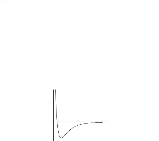
u(ri − rj) = u(r) is the interaction energy and U the potential of the box walls. The particles are polarizable and this leads to an attractive van der Waals interaction between the induced electric dipole moments. Such an interaction energy is proportional to r−6, where r is the interatomic distance. At short distances, however, the electrons repel because of the Pauli exclusion principle. Although the repulsive potential energy usually decays exponentially with r, we will write it in the form:

(2r0 is the minimal distance to which the particles of ”hard-core” radius r0 can approach.)

The partition function of N interacting identical particles is

Figure 2.1: Interatomic potential energy u(r) in real gases.

After integrating over all momenta, the partition function becomes:

where ZI carries all the interactions between the particles. We calculate the partition function in a mean-field approximation in which all the correlations are neglected. The potential acting on one particle is calculated by assuming a uniform

14

Phase transitions

spatial distribution of other particles,

V −Nb. Here we subtracted from V the volume occupied by other particles. N/2 is the number of pairs of particles. The mean-field potential Φ is:

This is the familiar van der Waals equation. We derived the van der Waals equation of state in a mean-field approximation, we neglected all the correlations between the molecules. Nevertheless, this equation qualitatively correctly describes the liquid-gas transition and it also predicts the existence of the critical point. However, as we neglected the correlations, which are essential in the vicinity of the critical point, it does not predict the correct critical behaviour.

15

Phase transitions

Below the critical point, the liquid and the gas phases are separated by a first order phase transition. The equilibrium transition between the two phases takes place when their chemical potentials and therefore the Gibbs free energies are equal.

Some comments are in place here.

•Critical exponents. The van der Waals equation was derived in a mean-fiel approximation, therefore all the exponents are mean-field like.

•Liquid → gas transition. The liquid phase is stable until the point A is reached. In equilibrium, at this point, liquid starts to evaporate, the system enters the coexistence region (mixture of gas and liquid) until the point B is reached, which corresponds to the pure gas phase.

If equilibrium is not reached, the liquid phase persists beyond the point A towards the point D. In this region, the liquid is metastable and can (at least in principle) persist until the point D is reached. Beyond this point, the compressibility is negative, the liquid state is unstable (not accessible).

•Gas → liquid transition. The situation is reversed. In equilibrium, the gas phase is stable until the point B is reached. This is the onset of the coexistence region which exists until the point A is reached. Metastable gas phase exists between the points B and E and, again, the region E to D is unstable.

•Convexity. As we have discussed in Section 2.3.3 already, the Helmholtz free energy F of a stable system has to be a concave function of V . For metastable states it is concave locally whereas for unstable states, it is convex.

15

Phase transitions

•Spinodals. The transition from a metastable (homogeneous) state toward the equilibrium (mixed) state is connected with the nucleation of droplets of the new phase. Droplets firs nucleate and then grow until the equilibrium (coexistence) is reached between the new and the old phase. Nucleation is a dynamic process.

The ultimate stability limit of the metastable state is called the spinodal line. Along this line the isothermal compressibility diverges, therefore the spinodal line is in a sense a line of critical points. In the van der Waals (meanfield) systems the separation between the metastable and unstable states is sharp. Beyond MFA, for systems with short-range correlations, however, the transition between metastable and unstable states is often gradual.

Ising model

The Ising model is the prototype model for all magnetic phase transitions and is probably the most studied model of statistical physics. In this model, the spin

operator ~ is replaced by a number, which represents the − component of the

Sb z

spin and is usually S = ±1 (”up” or ”down”). The order parameter m = hSi is thus one-dimensional, it is a two-component scalar.

The Ising Hamiltonian is

Jij is the interaction energy between the spins i and j. Usually (not always) the sum is only over nearest neighbouring (NN) pairs, then Jij = J. H is the external magnetic field (in energy units). The case J > 0 corresponds to ferromagnetism and J < 0 to antiferromagnetism. As we shall show later, the Ising model has a phase transition at finit T if d > 1. In d = 1 the transition is at T = 0. Therefore we say that d = 1 is the lower critical dimension of the Ising model.

In the low-temperature phase, the symmetry is broken, the spins are ordered, the order parameter is m 6= 0, whereas in the high-temperature phase the symmetry is not broken, m vanishes, the spins are disordered. Therefore this model is a prototype of all order-disorder transitions. Other examples of order-disorder transitions, I would like to mention, are lattice gases and binary alloys. All these systems are equivalent to each other, they all have the same critical behaviour (which of course depends on d), for given d they all belong to the same universality class.

16

Phase transitions

Lattice gas

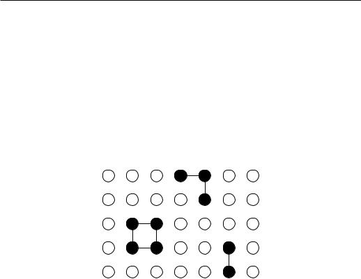
Imagine that a fluid (gas or liquid) system is divided into a regular lattice of cells of volume roughly equal to the particle (atom, molecule) volume. We say that the cell is occupied if a particle centre falls into this cell. Since the cell volume is comparable to the particle volume, there can be not more than one particle per cell. Notice that microscopic details (like positions of the particles) are irrelevant in the critical region, therefore the lattice gas model is suitable for studying the critical behaviour of real gases although the space is discretized. (It is also assumed that the kinetic energy of the gas particles, which is neglected in the lattice gas model, does not contribute a singular part to the partition function.)

Figure 2.2: A configuration of a lattice gas in d = 2. Solid circles represent atoms and open circles empty sites. Lines show bonds between nearest–neighbouring atoms.

A lattice gas is thus a collection of particles whose kinetic energy is neglected and that are arranged into discrete cells. The cells are either occupied by one atom [closed circles in Fig. 2.2] or empty [open circles]. The Hamiltonian is:

where u is the interaction potential,

and hi, ji is the sum over pairs. pi is the occupation number, it is 1 if the site is occupied by an atom, and zero otherwise. The occupation is, like the Ising spin,

17

Phase transitions

a double-valued function. Therefore we expect that the two models are related. Indeed, if we set

Here, z is the number of NN neighbours (4 for square lattice, 6 for simple cubic lattice), and H0 is a constant, independent of S. Thus, we see that Hlg is identical to the Ising Hamiltonian if we set u/4 = J and (µ/2 + uz/4) = H. For u > 0, the atoms attract and they ”condense” at low temperatures whereas for u < 0 the atoms repel. At 1/2 coverage (one half of the lattice sites is occupied) and u < 0, the empty and occupied sites will alternate at low T , like spins in an antiferromagnet.

The lattice gas model in d = 2 is used to investigate, e.g., hydrogen adsorbed on metal surfaces. The substrate provides discrete lattice sites on which hydrogen can be adsorbed. By varying the pressure, the coverage (amount of adsorbed hydrogen) is varied. This corresponds to varying the fiel in magnetic systems.

There is an important difference between the lattice gas and the Ising models of magnetism. The number of atoms is constant (provided no atoms evaporate from or condense on the lattice), we say that the order parameter in the lattice gas models is conserved whereas it is not conserved in magnetic systems. This has important consequences for dynamics.

Binary alloys

A binary alloy is composed of two metals, say A and B, arranged on a lattice. We introduce the occupations:

18

Phase transitions

Depending on which atoms are nearest neighbours, there are three different NN interaction energies: uAA, uBB, and uAB = uBA. The Hamiltonian is:

where each sum hi, ji runs over all NN pairs. If we write pi = (1 + Si)/2 and

H0 is a constant, and J = (uAA + uBB − 2uAB)/4. For binary alloys, the order parameter is also conserved.

Ising model in d = 1

It is not difficul to solve the Ising model in the absence of H in d = 1 exactly. The Hamiltonian of a linear chain of N spins with NN interactions is

H1d = −J X SiSi+1. (2.23)

i

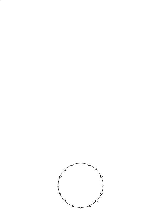
We shall use periodic boundary conditions, that means that the spins will be

N 1 2

3

i+1

i

Figure 2.3: Lattice sites of an Ising model in one dimension with periodic boundary conditions.

19