

Figure A-9 The two measures differ only for the direction of the cross-filter. The results are completely different.
The definitions of the two measures are as follows:
Click here to view code image
CustomerCount := COUNTROWS ( Customer )
CustomerFiltered := CALCULATE (
COUNTROWS ( Customer ),
CROSSFILTER ( Customer[CustomerKey], Sales[Custo
)
You can see that CustomerCount uses the default filtering. Thus, Product filters Sales, but Sales does not filter Customer. In the second measure, on the other hand, the filter flows from Product to Sales and then reaches Customer, so the formula counts only the customers who bought one of the filtered products.
Different types of models
In a typical model, there are many tables linked through relationships. These tables can be classified using the following names, based on their usage:

 Fact table A fact table contains values that you want to aggregate. Fact tables typically store events that happened in a specific point in time and that can be measured. Fact tables are generally the largest tables in the model, containing tens of millions or even hundreds of millions of rows. Fact tables normally store only numbers—either keys to dimensions or values to aggregate.
 Dimension A dimension is useful to slice facts. Typical dimensions are products, customers, time, and categories. Dimensions are usually small tables, with hundreds or thousands of rows. They tend to have many attributes in the form of strings because their main purpose is to slice values.
 Bridge tables Bridge tables are used in more complex models to represent many-to-many relationships. For example, a customer who might belong to multiple categories can be modeled with a bridge table that contains one row for each of the categories of the customer.
Star schema
When you look at the diagram of your model, if it is built based only on fact tables and dimensions, you can put the fact table in the center with all the dimensions around it—an arrangement known as a star schema, as shown in Figure A-10.

Figure A-10 A star schema emerges if you put the fact table in the middle and all the dimensions around it.
Star schemas have a lot of great features: They are fast and easy to understand and manage. As you read in this book, you will see that they are—with good reason—the foundation of most analytical databases. Sometimes, however, you need to structure your model in different ways, the most common of which are described in the next sections.
Snowflake schema
Sometimes, a dimension is linked to another dimension that further classifies it. For example, products might have categories, and you might decide to store the categories in a separate table. As another example, stores can be divided in business units, which again, you might decide to store in a separate table. As an example, Figure A-11 shows products that, instead of having the category name as a column, store a category key, which, in turn, refers to the Category table.
Figure A-11 Categories are stored in their own table, and Product refers to that table.
If you use such a schema, both product categories and business units are still dimensions, but instead of being related directly to the fact table, they are related through an intermediate dimension. For example, the Sales table contains the ProductKey column, but to obtain the category name, you must reach Product from Sales and then Category from Product. In such a case, you obtain a different schema, which is known as a snowflake, as shown in Figure A-12.
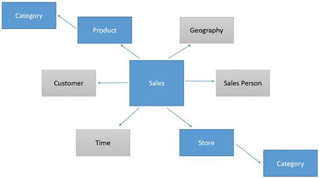
Figure A-12 A snowflake is a star schema with additional dimensions linked to the original dimensions.
Dimensions are not related among themselves. For example, you can think of the relationship between Category and Sales as a direct relationship, but it is passing through the Store table. For no reason is a relationship allowed to link Store with Geography. In such a case, in fact, the model would become ambiguous because there would be multiple paths from Sales to Geography.
Snowflake schemas are somewhat common in the business intelligence (BI) world. Apart from a slight degradation of performance, they are not a bad choice. Nevertheless, whenever possible, it is better to avoid snowflakes and stick to the more standard star schema because the DAX code tends to be easier to develop and less error-prone.
Models with bridge tables
A bridge table typically lies between two dimensions to create many-to-many relationships between the dimensions. For example, Figure A-13 shows how an individual customer might belong to multiple categories. Marco belongs both to the Male and Italian categories, whereas Kate belongs only to the Female category. If you have a scenario like this, then you design two relationships starting from the bridge and reaching, respectively, Customer and Category.
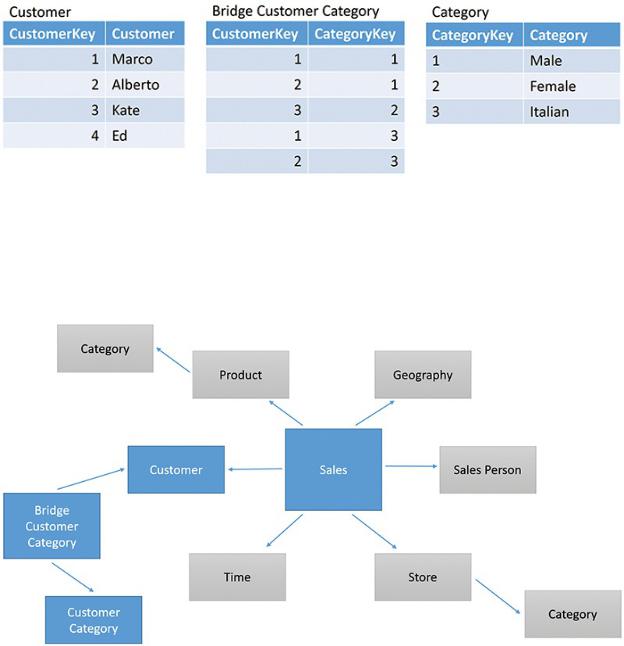
Figure A-13 A bridge table lets an individual customer belong to different categories.
When your model contains bridge tables, it takes a new shape that has never been named in the BI community. Figure A-14 shows an example where we added the capability for a customer to belong to multiple customer categories.
Figure A-14 A bridge table links two dimensions, but it is different from a regular snowflake.
The difference between the regular snowflake schema and this one with a bridge table is that this time, the relationship between Customer Category and Sales is not a straight relationship that passes through two dimensions. In fact, the relationship between Customer and the bridge is in the opposite direction. If it was going from the Customer to the bridge, then it would have been a snowflake. Because of its direction (which reflects its intended usage) it becomes a many-to-