

then using the dimension at the minute level is a waste of space and time. If you store the dimension at the half-hour level, the whole dimension will use 48 rows instead of 1,440. This gives you two orders of magnitude and a tremendous saving in terms of RAM and query speed because of the savings applied to the larger fact table. Figure 7-6 shows you the same time dimension as Figure 7-5, but in this case, it is stored at the half-hour level.
Of course, if you store the time at the half-hour level, you will need to compute a column in the fact table that acts as an index for the table. In Figure 7-6, we used Hours × 60 + Minutes as the index instead of using a simple auto-increment column. This makes it much easier to compute the time key in the fact table, by starting from the date/time. You can obtain it by using simple math, without the need to perform complex ranged lookups.
FIGURE 7-6 By storing at the half-hour level, the table becomes much smaller.
Let us repeat this very important fact: Date and time must be stored in separate columns. After many years of consulting different customers with different needs, we have yet to find many cases where storing a single date/time column is the best solution. This is not to say that it is forbidden to store a date/time column. In very rare cases, using a date/time column is the only viable option. However, it is so rare to find a good case for a date/time column that we always default to splitting the columns—although we are ready to change our minds if (and only if) there is a strong need to do so. Needless to say, this does not typically happen.
Intervals crossing dates
In the previous section, you learned how to model a time dimension. It is now time to go back to the introduction and perform a deeper analysis of the scenario in which events happen, and they have a duration that might span to the next day.

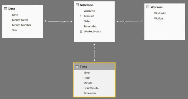
As you might recall, we had a Schedule table that contained the worked hours. Because a worker might start a shift in the late evening (or even at night), the working day could span to the next day, making it difficult to perform analysis on it. Let us recall the data model, which is shown in Figure 7-7.
FIGURE 7-7 This figure shows a simple data model for handling working schedules.
First, let us see how to perform the analysis on this model in the right way by using some DAX code. Be aware that using DAX is not the optimal solution. We use this example only to show how complex the code might become if you do not work with the correct model.
In this very specific example, a shift might span over two days. You can obtain the real working hours by first computing the working hours in the day and then removing from the day the shift hours that might be in the next day. After this first step, you must sum the potential working hours of the previous day that spanned to the current day. This can be accomplished by the following DAX code:
Click here to view code image
Real Working Hours =
--
-- Computes the working hours in the same day
--
SUMX ( Schedule, IF (
Schedule[TimeStart] + Schedule[HoursWorked] Schedule[HoursWorked],
( 1 - Schedule[TimeStart] ) * 24
)
)
--
-
- Check if there are hours today, coming from a pre
--
+ SUMX (
VALUES ( 'Date'[Date] ), VAR
CurrentDay = 'Date'[Date] RETURN
CALCULATE ( SUMX (
Schedule, IF (
Schedule[TimeStart] + Schedule[H
Schedule[HoursWorked] - ( 1 - Sc
)
),
'Date'[Date] = CurrentDay - 1
)
)
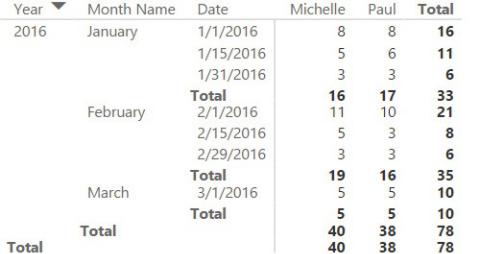
Now the code returns the correct number, as shown in Figure 7-8.
FIGURE 7-8 The new measure shows the working hours in the correct day.
The problem appears to have been solved. However, at this point, the real question is whether you really want to write such a measure. We had to because we are writing a book and we needed to demonstrate how complex it is, but you are not, and you might have better options. The chances of making mistakes with such a complex piece of code are very high. Moreover, this works only in the very
special case in which an event spans two consecutive days. If an event has a duration of more than two days, this code becomes much more complex, thus increasing the chances of making mistakes.
As is usually the case in this book (and in the real world), the solution is not writing complex DAX code. The best solution is to change the data model so that it reflects, in a more precise way, the data you need to model. Then, the code will be simpler (and faster).
There are several options for changing this model. As we anticipated earlier in this chapter, the problem is that you are storing data at the wrong granularity level. In fact, you must change the granularity if you want to be able to slice by the hours the employees actually worked in a day and if you are considering the night shift as belonging to the calendar day. Instead of storing a fact that says, “Starting on this day, the worker worked for some hours,” you must store a fact that says, “On this given day, the worker worked for so many hours.” For example, if a worker starts a shift on September 1st and ends it on September 2nd, you will store two rows: one with the hours on September 1st and one with the hours on September 2nd, effectively splitting the single row into multiple ones.
Thus, an individual row in the previous fact table might as well be transformed into multiple rows in the new data model. If a worker starts a shift during the late evening, then you will store two rows for the shift—one for the day when the work started, with the correct starting time, and another on the next day, starting at midnight, with the remaining hours. If the shift spans multiple days, then you can generate multiple rows. This, of course, requires a more complicated data preparation, which we do not show in the book because it involves quite complex M code. However, you can see this in the companion content, if you are interested. The resulting Schedule table is shown in Figure 7-9, where you can see several days starting at midnight, which are the continuation of the previous days. The hours worked have been adjusted during Extract, Transform, Load (ETL).

FIGURE 7-9 The Schedule table now has a lower granularity at the day level.
Because of this change in the model, which is correcting the granularity, now you can easily aggregate values by using a simple SUM. You will obtain the correct result and will avoid the complexity shown in the previous DAX code.
A careful reader might notice that we fixed the field containing HoursWorked, but we did not perform the same operation for Amount. In fact, if you aggregate the current model that shows the sum of the amount, you will obtain a wrong result. This is because the full amount will be aggregated for different days that might have been created because of midnight crossing. We did that on purpose because we wanted to use this small mistake to investigate further on the model.
An easy solution is to correct the amount by simply dividing the hours worked during the day by the total hours worked in the shift. You should obtain the percentage of the amount that should be accounted for the given day. This can be done as part of the ETL process, when preparing the data for analysis. However, if you strive for precision, then it is likely that the hourly rate is different depending on the time of the day. There might be shifts that mix different hourly rates. If this is the case, then, again, the data model is not accurate enough.
If the hourly price is different, then you must change, again, the data model to a lower level of granularity (that is, a higher level of detail) by moving the granularity to the hourly level. You have the option of making it easy by storing one fact per hour, or by pre-aggregating values when the hourly rate does not
change. In terms of flexibility, moving to the hourly level gives you more freedom and easier-to-produce reports because, at that point, you also have the option of analyzing time across different days. This would be much more complex in a case where you pre-aggregate the values. On the other hand, the number of rows in the fact table grows if you lower the granularity. As is always the case in data modeling, you must find the perfect balance between size and analytical power.
In this example, we decided to move to the hourly level of granularity, generating the model shown in Figure 7-10.
FIGURE 7-10 The new measure shows the working hours in the correct day.
In this new model, the fact basically says, “This day, at this hour, the employee worked.” We increased the detail to the lowest granularity. At this point, computing the number of hours worked does not even require that we perform a SUM. In fact, it is enough to count the number of rows in Schedule to obtain the number of worked hours, as shown in the following WorkedHours measure:
Click here to view code image
WorkedHours := COUNTROWS ( Schedule )
In case you have a shift starting in the middle of the hour, you can store the number of minutes worked in that hour as part of the measure and then aggregate using SUM. Alternatively, in very extreme cases, you can move the granularity to a lower level—to the half-hour or even the minute level.