


Sales[ProductName],
Sales[ColorName],
Sales[Manufacturer],
Sales[BrandName],
Sales[ProductCategoryName],
Sales[ProductSubcategoryName]
), ALL (
Purchases[ProductName],
Purchases[ColorName],
Purchases[Manufacturer],
Purchases[BrandName],
Purchases[ProductCategoryName],
Purchases[ProductSubcategoryName]
)
)
)
This calculated table performs two ALL operations on product columns from Sales and Purchases, reducing the number of columns and computing the distinct combinations of the required data. Then it uses UNION to merge them together. Finally, it uses DISTINCT to remove further duplicates, which are likely to appear because of the UNION function.
 Note
Note
The choice between using M or DAX code is entirely up to you and your personal taste. There are no relevant differences between the two solutions.
Once again, the correct solution to the model is to restore a star schema. This simple concept bears frequent repetition: Star schemas are good, but everything else might be bad. If you are facing a modeling problem, before doing anything else, ask yourself if you can rebuild your model to move toward a star schema. By doing this, you will likely go in the right direction.
Filtering across dimensions
In the previous example, you learned the basics of multiple dimension handling.

There, you had two over-denormalized dimensions and, to make the model a better one, you had to revert to a simpler star schema. In this next example, we analyze a different scenario, again using Sales and Purchases.
You want to analyze the purchases of only the products sold during a given period—or, more generally, the products that satisfy a given selection. You learned in the previous section that if you have two fact tables, the best way to model the scenario is to relate them to dimensions. That would give you the ability to use a single dimension to filter both. Thus, the starting scenario is the one shown in Figure 3-5.
FIGURE 3-5 In this model, two fact tables are related to two dimensions.
Using this model and two basic measures, you can easily build a report like the one shown in Figure 3-6, where you can see both the sales and purchases divided by brand and year.

FIGURE 3-6 In this simple star schema, sales and purchases divided by year and brand are computed easily.
A more difficult calculation is to show the number of purchases for only the products that are being sold. In other words, you want to use Sales as a filter to further refine the products so that any other filter imposed on sales (the date, for example) restricts the list of products for which you are computing purchases.
There are different approaches to handling this scenario. We will show you some of them and discuss the advantages and disadvantages of each solution.
If you have bidirectional filtering available in your tool (at the time of this writing, bidirectional filtering is available in Power BI and SQL Server Analysis Services, but not in Excel), you might be tempted to change the data model that enables bidirectional filtering on Sales versus Product so that you see only the products sold. Unfortunately, to perform this operation, you must disable the relationship between Product and Purchases, as shown in Figure 3-7. Otherwise, you would end up with an ambiguous model, and the engine would refuse to make all the relationships bidirectional.
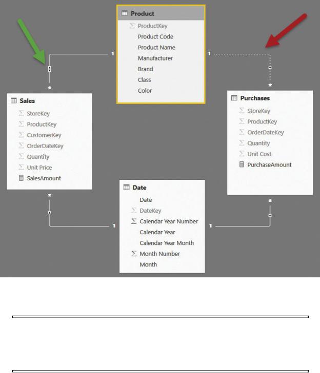
FIGURE 3-7 To enable bidirectional filtering between the Sales and Product tables, you must disable the relationship between Product and Purchases.
 Info
Info
The DAX engine refuses to create any ambiguous model. You will learn more about ambiguous models in the next section.
If you follow the filtering options of this data model, you will quickly discover that it does not solve the problem. If you place a filter on the Date table, for example, the filter will propagate to Sales, then to Product (because bidirectional filtering is enabled), but it will stop there, without having the option of filtering Purchases. If you enable bidirectional filtering on Date, too, then the data model