

Chapter 6. Using snapshots
A snapshot is a kind of table that is often used in the modeling of data. In the first chapters of this book, you became familiar with the idea of dividing a model by fact tables and dimensions, and you learned that a fact is a type of event—that is, something that happens. Then, you aggregated values from the fact table by using an aggregation function, like SUM, COUNT or DISTINCTCOUNT. But the truth is, sometimes a fact is not an event. Sometimes, a fact stores something that has been measured, like the temperature of an engine, the daily average number of customers who entered a store each month, or the quantity on-hand of a product. In all these cases, you store a measurement at a point in time instead of the measure of an event. All these scenarios are typically modeled as snapshots. Another kind of snapshot is the balance of a current account. The fact is an individual transaction in the account, and a snapshot states what the balance was, at a given point in time.
A snapshot is not a fact. It is a measure taken at some point in time. In fact, when it comes to snapshots, time is a very important part of the equation. Snapshots might appear in your model because the more granular information is too large or it is unavailable.
In this chapter, we analyze some kinds of snapshots to give you a good level of understanding on how to handle them. As always, keep in mind that your model is likely to be slightly different from anything we will ever be able to describe as a standard pattern. Be prepared to adjust the content of this book to your specific needs, and use some creativity in developing your model.
Using data that you cannot aggregate over time
Suppose you periodically perform an inventory in your stores. The table that contains the inventory is a fact table. However, this time, the fact is not something that happened; it is something that holds true at a given point in time. What you are saying in the fact table is, “at this date, the quantity of this product available in this store is x.” The next month, when you perform the same operation, you can state another fact. This is a snapshot—that is, a measure of what was available at that time. From an operational point of view, the table is a fact table because you are likely to compute values on top of the table, and because the table is linked to dimensions. The difference here has more to do with the nature of the fact than with the structure.
Another example of a snapshot is the exchange rate of a currency. If you need to store the exchange rate of a currency, you can store it in a table that contains the date, the currency, and its value compared to some other reference currency, like USD. It is a fact table because it is related to dimensions, and it contains numbers that you will use for an aggregation. However, it does not store an event that happened. Rather, it stores a value that has been measured at a given point in time. We will provide a complete lesson of how to manage exchange rates later in Chapter 11, “Working with multiple currencies.” For the purposes of this chapter, it is enough to note that a currency exchange rate is a kind of snapshot.
It is useful to differentiate between the following kinds of snapshots:
 Natural snapshots These are data sets in which the data is, by its nature, in the form of a snapshot. For example, a fact table that measures the temperature of the water in an engine on a daily basis is a natural snapshot. In other words, the fact is the measure, and the event is the measurement.
 Derived snapshots These are data sets that look like snapshots, but are treated as such only because we tend to think of them as snapshots. Think, for example, of a fact table that contains the balance of the current accounts on a monthly basis. Every month, the measure is the balance, but in reality, the balance of the account is derived from the sum of all the transactions (either positive or negative) that previously occurred. Thus, the data is in the form of a snapshot, but it can also be computed by a simpler aggregation of the raw transactions.
The difference is important. In fact, as you will learn in this chapter, handling snapshots comes with both advantages and disadvantages. You must find the correct balance between them to choose the best possible representation for your data. Sometimes, it is better to store balances; other times, it is better to store transactions. In the case of derived snapshots, you have the freedom (and the responsibility) to make the right choice. With natural snapshots, however, the choice is limited, because the data comes in naturally as a snapshot.
Aggregating snapshots
Let us start the analysis of snapshots by learning the details on how to correctly aggregate data from snapshots. As an example, let us consider an Inventory fact that contains weekly snapshots of the on-hand quantity for each product and store. The full model is shown in Figure 6-1.

FIGURE 6-1 The Inventory table contains snapshots of on-hand quantity, created on a weekly basis.
Initially, this looks like a simple star schema with two fact tables (Sales and Inventory) and no issues at all. Indeed, both fact tables have the same day, product, and store granularity dimensions. The big difference between the two tables is that Inventory is a snapshot, whereas Sales is a regular fact table.
 Note
Note
As you will learn in this section, computing values on top of snapshot tables hides some complexity. In fact, in the process of building the correct formula, we will make many mistakes, which we will analyze together.
For now, let us focus on the Inventory table. As we mentioned, Inventory contains weekly snapshots of the on-hand quantity for every product and store.

You can easily create a measure that aggregates the On Hand column by using the following code:
Click here to view code image
On Hand := SUM ( Inventory[OnHandQuantity] )
Using this measure, you can build a matrix report in Power BI Desktop to analyze the values for an individual product. Figure 6-2 shows a report with the details of one type of stereo headphones in different stores in Germany.
FIGURE 6-2 This report shows the on-hand quantity for one product in different stores in Germany.
Looking at the totals in the report, you can easily spot the problem. The total for each store at the year level is wrong. In fact, if in the Giebelstadt store there were 18 headphones available in November and none in December, then the total value for 2007 is obviously not 56. The correct value should be zero, as there were none on-hand after November 2007. Because the snapshot is a weekly one, if you expand the month to the date level, you will notice that even at the month level, the value reported is incorrect. You can see this in Figure 6-3, where the total at the month level is shown as the sum of the individual date values.

FIGURE 6-3 The total at the month level is generated by summing the individual dates, resulting in an incorrect value.
When handling snapshots, remember that snapshots do not generate additive measures. An additive measure is a measure that can be aggregated by using SUM over all the dimensions. With snapshots, you must use SUM when you aggregate over the stores, for example, but you cannot use SUM to aggregate over time. Snapshots contain sets of information that are valid at a given point in time. However, at the grand-total level, you typically don’t aggregate over dates by using a sum—for example, showing the sum of all the individual days. Instead, you should consider the last valid value, the average, or some other kind of aggregation to display a meaningful result.
This is a typical scenario in which you must use the semi-additive pattern, where you show the values from the last period for which there is some information. If you focus on April, for example, the last date for which there is data is the 28th. There are multiple ways to handle this calculation by using DAX. Let us explore them.
The canonical semi-additive pattern uses the LASTDATE function to retrieve the last date in a period. Such a function is not useful in this example because, when you select April, LASTDATE will return the 30th of April, for which there is no data. In fact, if you modify the On Hand measure with the following code, the result will clear out the monthly totals:
Click here to view code image
On Hand :=
CALCULATE (
SUM ( Inventory[OnHandQuantity] ), LASTDATE ( 'Date'[Date] )
)
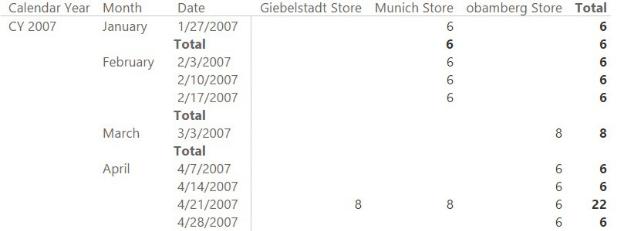
You can see this in Figure 6-4, where the totals at the month level are blank.
FIGURE 6-4 If you use LASTDATE to retrieve the last date in a period, the totals disappear.
The date you need to use is the last date for which there is data, which might not correspond to the last date of the month. In this case, DateKey in the Inventory table is a date, so you might try a different formulation. Instead of using LASTDATE on the Date table, which contains all the dates, you might be tempted to use LASTDATE on the Inventory date column in the Inventory table, which contains only the available dates. We have seen these kinds of formulas multiple times in naïve models. Unfortunately, however, they result in incorrect totals. This is because it violates one of the best practices of DAX, that is to apply filters on dimensions instead of applying them on the fact table, for columns belonging to a relationship. Let us analyze the behavior by looking at the result in Figure 6-5, where the measure has been modified with the following code:
Click here to view code image
On Hand :=
CALCULATE (
SUM ( Inventory[OnHandQuantity] ),
LASTDATE ( Inventory[DateKey] )
)
FIGURE 6-5 Using LASTDATE on the Inventory date column still results in wrong numbers.
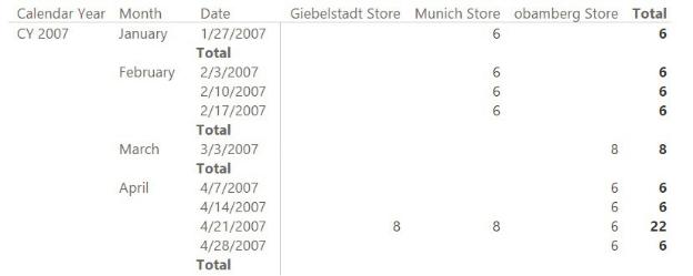
Look at the totals for April. Notice that in Giebelstadt and Munich, the value shown is from the 21st of April, whereas for Obamberg, the value is from the 28th. However, the grand total for all three stores is only 6, which matches the total of the values for all three stores on the 28th. What is happening? Instead of counting the values from the last date for Munich and Giebelstadt (the 21st) and the value for the last date for Obamberg (the 28th), the grand total counts only the values from the 28th because that is the last date among the three stores. In other words, the value given—that is, 6—is not the grand total, but rather the partial total at the store level. In fact, because there are no quantities on the 28th for Giebelstadt and Munich, their monthly total should show a zero, not the last available value. Thus, a correct formulation of the grand total should search for the last date for which there are values for at least one shop. The standard solution for this pattern is as follows:
Click here to view code image
On Hand := CALCULATE (
SUM ( Inventory[OnHandQuantity] ), CALCULATETABLE (
LASTNONBLANK ( 'Date'[Date], NOT ( ISEMPTY ( ALL ( Store )
)
)
Or, in this specific case, as follows:
Click here to view code image
On Hand := CALCULATE (
SUM ( Inventory[OnHandQuantity] ), LASTDATE (
CALCULATETABLE (
VALUES ( Inventory[Date] ), ALL ( Store )
)
)
)
Both versions work fine. You decide which one to use depending on the data distribution and some peculiarities of the model, which are not worth investigating here. The point is that using this version of the on-hand calculation, you obtain the desired result, as shown in Figure 6-6.
FIGURE 6-6 The last formula yields the correct results at the total level.
This code runs just fine, but it has one major drawback: It must scan the Inventory table whenever it searches for the last date for which there is data. Depending on the number of dates in the table, and on data distribution, this might take some time, and could result in poor performance. In such a case, a good solution is to anticipate the calculation of which dates are to be considered valid dates for the inventory at process time when your data is loaded in memory. To do this, you can create a calculated column in the Date table that indicates whether the given date is present in the Inventory table. Use the following code:
Click here to view code image
Date[RowsInInventory] := CALCULATE ( NOT ISEMPTY (
Inventory ) )
The column is a Boolean with only two possible values: TRUE or FALSE. Moreover, it is stored in the Date table, which is always a tiny table. (Even if you had 10 years of data, the Date table would account for only around 3,650 rows.) The consequence of this is that scanning a tiny table is always a fast operation, whereas scanning the fact table—which potentially contains millions of rows— might not be. After the column is in place, you can change the calculation of the on-hand value as follows:
Click here to view code image
On Hand := CALCULATE (
SUM ( Inventory[OnHandQuantity] ), LASTDATE (
CALCULATETABLE (
VALUES ( 'Date'[Date] ), 'Date'[RowsInInventory] = TRUE
)
)
)
Even if the code looks more complex, it will be faster because it needs to search for the inventory dates in the Date table, which is smaller, filtering by a Boolean column.
This book is not about DAX. It is about data modeling. So why did we spend so much time analyzing the DAX code to compute a semi-additive measure? The reason is that we wanted to point your attention to the following details, which do in fact relate to data modeling:
 A snapshot table is not like a regular fact table Its values cannot be summed over time. Instead, they must use non-additive formulas (typically
LASTDATE).
 Snapshot granularity is seldom that of the individual date A table snapshotting the on-hand quantity for each product every day would quickly turn into a monster. It would be so large that performance would be very bad.
 Mixing changes in granularity with semi-additivity can be problematic
The formulas tend to be hard to write. In addition, if you do not pay attention to the details, performance will suffer. And of course, it is very easy to