

1.You defined the new granularity of the SCD. The new granularity depended on the attributes of the dimension that were expected to change over time.
2.You modified the dimension so it used the right granularity. This required complex queries and, most importantly, the definition of a new customer code to use as the foundation of the relationship.
3.You modified the fact table so that it used the new code. Because the new code could not be easily computed, you had to search for its value in the new dimension by performing a lookup. All the slowly changing attributes were used to define the granularity.
We went through the whole process of describing how to handle SCDs with the Query Editor of Power BI Desktop. (You can perform the same steps in Excel 2016.) We wanted to show the level of complexity involved in handling SCDs. The next section describes rapidly changing dimensions. As you will discover, the management of rapidly changing dimensions is far simpler than that of SCDs. However, rapidly changing dimensions are not the optimal solution from a storage and performance point of view. Also, you can safely use the easier pattern of rapidly changing dimensions for slowly changing ones if your data model is small enough (that is, in the range of a few million rows).
Rapidly changing dimensions
As their name implies, slowly changing dimensions typically change slowly and do not produce too many versions of the entity they represent. We deliberately used customers under different sales managers as an example of an SCD that might potentially change every year. Because the changing attribute is owned by all customers, the number of new versions created is somewhat high. A more traditional example of an SCD might be tracking the current and historical address of a customer, as customers are not generally expected to update their address every year. We chose to use the sales manager example rather than the address one because the resulting model can be easily created with Excel or Power BI Desktop.
Another attribute that you might be interested in tracking—one that always changes each year—is the customer’s age. For example, suppose you want to analyze sales by age range. If you do not handle the customer’s age as an SCD, you cannot store it in the customer dimension. The customer’s age changes, and you need to track the age when the sale was made rather than the current age. You could use the pattern described in the previous section to handle age. However, this section shows a different way of handling changes in a dimension:
implementing the pattern for rapidly changing dimensions.
Suppose you have 10 years of data in your model. Chances are, if you have used SCDs, you have 10 different versions of the same customer in your table. If even more attributes must be monitored for changes, this number might easily increase up to a point where handling it becomes cumbersome. To address this, focus your attention on the fact that the whole dimension does not change. Rather, what changes is one attribute of the dimension. If an attribute changes too frequently, the best option is to store the attribute as a dimension by itself, which removes it from the customer dimension.
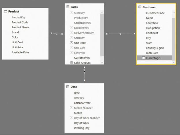
The starting model is shown in Figure 5-24, where the current age of the customer is saved in the Customer table.
FIGURE 5-24 The age of the customer is stored as an attribute of the Customer table.
The ages stored in the Customer table are the current ages of each customer. They are updated every day, based on the current date. But what about the
customer’s historical age—that is, his or her age when the sale was made? Because the customer’s age is changing quickly, a good way to model it is to store the historical age in the fact table by using a calculated column. Try the following code:
Click here to view code image
Sales[Historical Age] = DATEDIFF (
RELATED ( Customer[Birth Date] ), RELATED ( 'Date'[Date] ),
YEAR
)
At the time of the sale, this column computes the difference between the customer’s birth date and the date of the sale. The resulting value stores the historical age in a very simple and convenient way. If you store the data in the fact table and denormalize it there, you are not creating a dimension. This approach models the age without the whole process of data transformation that is required to handle an SCD.
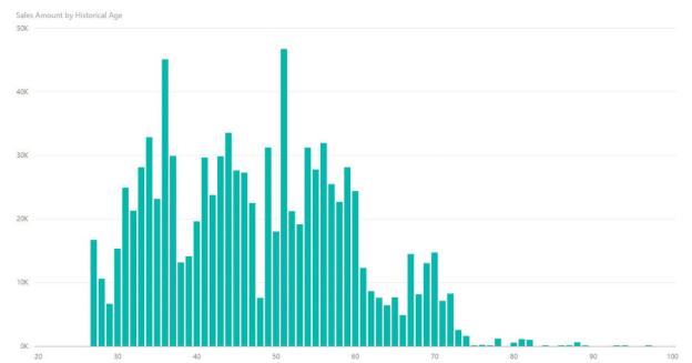
This column, alone, is already useful to build charts. For example, Figure 5-25 shows a histogram with the sales divided by age.
FIGURE 5-25 The historical age works perfectly fine to show histograms and charts.
The age, as a number, works fine for charts. But you might also be interested in grouping the age into different ranges to obtain different insights. In such a case, the best option is to create a real dimension and use the age in the fact table as a foreign key to point to the dimension. This will result in a data model like the one shown in Figure 5-26.
FIGURE 5-26 You can turn the historical age into a foreign key and build a proper age dimension.
In the Historical Age dimension, you can store age ranges or other interesting attributes. This enables you to build reports that slice by age range instead of an individual age. For example, the report shown in Figure 5-27 shows sales amount, the number of customers in that age range, and the average spent in that age range.