The energy of the waves increases with fetch:

where F is fetch.

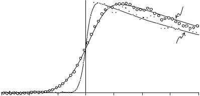
The jonswap spectrum is similar to the Pierson-Moskowitz spectrum except that waves continues to grow with distance (or time) as specified by the α term, and the peak in the spectrum is more pronounced, as specified by the γ term. The latter turns out to be particularly important because it leads to enhanced non-linear interactions and a spectrum that changes in time according to the theory of Hasselmann (1966).

Generation of Waves by Wind We have seen in the last few paragraphs that waves are related to the wind. We have, however, put o until now just how they are generated by the wind. Suppose we begin with a mirror-smooth sea (Beaufort Number 0). What happens if the wind suddenly begins to blow steadily at say 8 m/s? Three di erent physical processes begin:

1.The turbulence in the wind produces random pressure fluctuations at the sea surface, which produces small waves with wavelengths of a few centimeters (Phillips, 1957).

2.Next, the wind acts on the small waves, causing them to become larger. Wind blowing over the wave produces pressure di erences along the wave profile causing the wave to grow. The process is unstable because, as the wave gets bigger, the pressure di erences get bigger, and the wave grows faster. The instability causes the wave to grow exponentially (Miles, 1957).

3.Finally, the waves begin to interact among themselves to produce longer waves (Hasselmann et al. 1973). The interaction transfers wave energy from short waves generated by Miles’ mechanism to waves with frequencies slightly lower than the frequency of waves at the peak of the spectrum. Eventually, this leads to waves going faster than the wind, as noted by Pierson and Moskowitz.

16.5Wave Forecasting

Our understanding of ocean waves, their spectra, their generation by the wind, and their interactions are now su ciently well understood that the wave spectrum can be forecast using winds calculated from numerical weather models. If we observe some small ocean area, or some area just o shore, we can see waves generated by the local wind, the wind sea, plus waves that were generated in other areas at other times and that have propagated into the area we are observing, the swell. Forecasts of local wave conditions must include both sea and swell, hence wave forecasting is not a local problem. We saw, for example, that waves o California can be generated by storms more than 10,000 km away.

Various techniques have been used to forecast waves. The earliest attempts were based on empirical relationships between wave height and wave length and wind speed, duration, and fetch. The development of the wave spectrum

allowed evolution of individual wave components with frequency f travelling in direction θ of the directional wave spectrum ψ(f, θ) using

where ψ0 = ψ0(f, θ; x, t) varies in space (x) and time t, Si is input from the wind given by the Phillips (1957) and Miles (1957) mechanisms, Snl is the transfer among wave components due to nonlinear interactions, and Sd is dissipation.

The third-generation wave-forecasting models now used by meteorological agencies throughout the world are based on integrations of (16.39) using many individual wave components (The swamp Group 1985; The wamdi Group, 1988; Komen et al, 1996). The forecasts follow individual components of the wave spectrum in space and time, allowing each component to grow or decay depending on local winds, and allowing wave components to interact according to Hasselmann’s theory. Typically the sea is represented by 300 components: 25 wavelengths going in 12 directions (30◦). To reduce computing time, the models use a nested grid of points: the grid has a high density of points in storms and near coasts and a low density in other regions. Typically, grid points in the open ocean are 3◦ apart.

Some recent experimental models take the wave-forecasting process one step further by assimilating altimeter and scatterometer observations of wind speed and wave height into the model. Forecasts of waves using assimilated satellite data are available from the European Centre for Medium-Range Weather Forecasts.

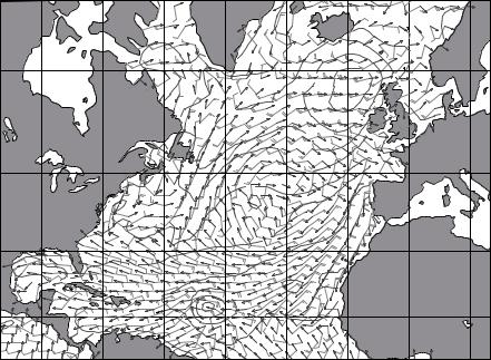
Noaa’s Ocean Modeling Branch at the National Centers for Environmental Predictions also produces regional and global forecasts of waves. The Branch use a third-generation model based on the Cycle-4 wam model. It accommodates ever-changing ice edge, and it assimilates buoy and satellite altimeter wave data. The model calculates directional frequency spectra in 12 directions and 25 frequencies at 3-hour intervals up to 72 hours in advance. The lowest frequency is 0.04177 Hz and higher frequencies are spaced logarithmically at increments of 0.1 times the lowest frequency. Wave spectral data are available on a 2.5◦× 2.5◦ grid for deep-water points between 67.5◦S and 77.5◦N. The model is driven using 10-meter winds calculated from the lowest winds from the Centers weather model adjusted to a height of 10 meter by using a logarithmic profile (8.20). The Branch is testing an improved forecast with 1◦× 1.25◦ resolution (figure 16.10).

16.6Measurement of Waves

Because waves influence so many processes and operations at sea, many techniques have been invented for measuring waves. Here are a few of the more commonly used. Stewart (1980) gives a more complete description of wave measurement techniques, including methods for measuring the directional distribution of waves.

Sea State Estimated by Observers at Sea This is perhaps the most common observation included in early tabulations of wave heights. These are the

Figure 16.10 Output of a third-generation wave forecast model produced by Noaa’s Ocean Modeling Branch for 20 August 1998. Contours are significant wave height in meters, arrows give direction of waves at the peak of the wave spectrum, and barbs give wind speed in m/s and direction. From noaa Ocean Modeling Branch.

significant wave heights summarized in the U.S. Navy’s Marine Climatological Atlas and other such reports printed before the age of satellites.

Satellite Altimeters The satellite altimeters used to measure surface geostrophic currents also measure wave height. Altimeters were flown on Seasat in 1978, Geosat from 1985 to 1988, ers–1 &2 from 1991, Topex/Poseidon from 1992, and Jason from 2001. Altimeter data have been used to produce monthly mean maps of wave heights and the variability of wave energy density in time and space. The next step, just begun, is to use altimeter observation with wave forecasting programs, to increase the accuracy of wave forecasts.

The altimeter technique works as follows. Radio pulse from a satellite altimeter reflect first from the wave crests, later from the wave troughs. The reflection stretches the altimeter pulse in time, and the stretching is measured and used to calculate wave height (figure 16.11). Accuracy is ±10%.

Accelerometer Mounted on Meteorological or Other Buoy This is a less common measurement, although it is often used for measuring waves during short experiments at sea. For example, accelerometers on weather ships measured wave height used by Pierson & Moskowitz and the waves shown in figure 16.2. The most accurate measurements are made using an accelerometer stabilized by a gyro so the axis of the accelerometer is always vertical.