

10.9. EULERIAN MEASUREMENTS |
179 |
months later the toys began washing ashore near Sitka, Alaska. A similar accident on May 27, 1990 released 80,000 Nike-brand shoes at 48◦N, 161◦W when waves washed containers from the Hansa Carrier.
The spills and eventual recovery of the toys and shoes proved to be good tests of a numerical model for calculating the trajectories of oil spills developed by Ebbesmeyer and Ingraham (1992, 1994). They calculated the possible trajectories of the spilled toys using the Ocean Surface Current Simulations oscurs numerical model driven by winds calculated from the Fleet Numerical Oceanography Center’s daily sea-level pressure data. After modifying their calculations by increasing the windage coe cient by 50% for the toys and by decreasing their angle of deflection function by 5◦, their calculations accurately predicted the arrival of the toys near Sitka, Alaska on November 16, 1992, ten months after the spill.
10.9Eulerian Measurements
Eulerian measurements are made by many di erent types of instruments on ships and moorings.
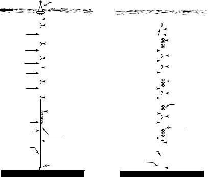
Moorings (figure 10.18) are placed on the sea floor by ships. The moorings may last for months to longer than a year. Because the mooring must be deployed and recovered by deep-sea research ships, the technique is expensive
Sea Surface
Wire
Wire
Wire
Nylon
Nylon
Wire 20m
Chafe Chain
5m
Chafe Chain
3m
Light, Radio, & Float
|
|
|
|
|
|
|
|
|
|
|
|
|
|
|
|
|
|
|
|
Sea Surface |
||||||||||||||||||||||
|
|
|
|
|
|
|
|
|
|
|
|
|
|
|
|
|
|
|
|
|
|
|
|
|
|
|
|
|
|
|
|
|
|
|
|
|
|
|
|
|
|
|
|
|
|
|
|
|
|
|
|
|
|
|
Chafe Chain |
|
|
|
|
|
|
|
|
|
|
|
|
|
|
|
|
|
|
|
|
|
|
|
|
|
|
|
|||
|
|
|
|
|
|
|
|
|
|
|
|
|
|
|
|
|
|
|
|
|
|
|
|
|
|
|
|
|
|
|
|
|
|
|
|
|
|
|
||||
|
|
|
|
|
|
|
|
|
|
|
|
|
|
|
|
|
|
|
|
|
|
|
|
|
|
|
|
|
|
|
|
|
|
|
|
|
||||||
|
|
|
|
|
|
|
|
|
|
|
|
|
|
|
|
|
|
|
|
|
|
|
|
|
|
|
|
|
|
|
|
|
|
|
|
|
|
|
||||
|
|
|
|
|
|
|
|
|
|
|
|
|
Instrument |
|
|
|
|
|
|
|
|
|
|
|
|
|
|
|
|
|
|
|
|
|
|
|
1/2" Chain |
|||||
|
|
|
|
|
|
|
|
|
|
|
|
|
|
|
Radio, Light, & Radio Float |
|
|
|
|
|
|
Wire (Typ. 20m) |
||||||||||||||||||||
|
|
|
|
|
|
|
|
|
|
|
|
|
|
|
|
|
|
|
|
|||||||||||||||||||||||
|
|
|
|
|
|
|
|
|
|
|
|
|
Instrument |
|
|
|
|
|
|
|
|
|
|
|
|
|
|
|
|
|
|
|
|
Top Buoyancy |
||||||||
|
|
|
|
|
|
|
|
|
|
|
|
|
|
|
|
|
Wire 20m |
|
|
|
|
|
|
|
|
|
|
|
|
|
(Typ. 20 shperes) |
|||||||||||
|
|
|
|
|
|
|
|
|
|
|
|
|
Instrument |
|
|
|
|
|
|
|
|
|
|
|
|
|
|
|
|
Instrument |
||||||||||||
|
|
|
|
|
|
|
|
|
|
|
|
|
|
|
|
|
|
|
|
|
|
|
|
|
|
|||||||||||||||||
|
|
|
|
|
|
|
|
|
|
|
|
|
|
Wire |
|
|
|
|
|
|
|
|
|
|
|
|
|
|
|
|
|
|
|
|
|
|||||||
|
|
|
|
|
|
|
|
|
Wire to 2000m |
|
Wire |
|
|
|
|
|
|
|
|
|
|
|
|
|
|
|
|
|
|
|
|
|
Instrument |
|||||||||
|
|
|
|
|
|
|
|
|
|
|
|
|
Instrument |
|
|
|
|
|
|
|
|
|
|
|
|
|
|
|
|
Intermediate Buoyancy |
||||||||||||
|
|
|
|
|
|
|
|
|
|
|
|
|
|
|
|
|
|
|
|
|
|
|
|
|
|
|||||||||||||||||
|
|
|
|
|
|
|
|
|
|
|
|
|
|
|
|
|
|
|
|
|
|
|
|
|
|
|
|
|
|
|
|
|
||||||||||
|
|
|
|
|
|
|
|
|
|
|
|
|
|
Wire 20m |
|
|
|
|
|
|
|
|
|
|
|
|
|
|
|
|
|
(Typ. 10 spheres) |
||||||||||
|
|
|
|
|
|
|
|
|
|
|
|
|
|
|
|
|
|
|
|
|
|
|
|
|
|
|
|
|
|
|
|
|
|
|||||||||
|
|
|
|
|
|
|
|
|
|
|
|
|
|
|
|
|
|
|
|
|
|
|
|
|
|
|
|
|
|
|
|
|
Instrument |
|||||||||
|
|
|
|
|
|
|
|
|
|
|
|
|
Instrument |
|
Wire |
|
|
|
|
|
|
|
|
|
|
|
|
|
|
|
|
|
|
|
|
|
||||||
|
|
|
|
|
|
|
|
|
|
|
|
|
|
|
|
|
|
|
|
|
|
|
|
|
|
|
|
|
|
|
|
|
|
|
|
Intermediate Buoyancy |
||||||
|
|
|
|
|
|
|
|
|
|
|
Backup-Recovery Section |
|
|
|
|
|
|
|
|
|
|
|
|
|
|
|
|
|
|
|
|
|
|
|
(Typ. 6 spheres) |
|||||||
|
|
|
|
|
|
|
|
|
|
|
6" or 7" glass spheres in |
|
Wire 20m |
|
|
|
|
|
|
|
|
|
|
|
|
|
Instrument |
|||||||||||||||
|
|
|
|
|
|
|
|
|
|
|
|
|
|
|
|
|
|
|
|
|
|
|
||||||||||||||||||||
|
|
|
|
|
|
|
|
|
|
|
hardhats on chain |
|
|
|
|
|
|
|
|
|
|
|
|
|
|
|
|
|
|
|
|
|
|
|
||||||||
|
|
|
|
|
|
|
|
|
|
|
|
Wire |
|
|
|
|
|
|
|
|
|
|
|
|
|
|
|
|
|
|
|
Backup Recovery |
||||||||||
|
|
|
|
|
|
|
|
|
|
|
(Typ. 35 Spheres) |
|
|
|
|
|
|
|
|
|
|
|
|
|
|
|||||||||||||||||
|
|
|
|
|
|
|
|
|
|
|
|
|
|
|
|
|
|
|
|
|
|
|
|
|
|
|
|
|
|
|
|
|
|
Bouyancy |
||||||||
|
|
|
|
|
|
|
|
|
|
|
|
|
|
|
|
|
|
|
|
|
|
|
|
|
|
|
|
|
|
|
|
|
|
|
|
|
|
|
||||
|
|
|
|
|
|
|
|
|
|
|
|
|
Acoustic Release |
|
Wire |
|
|
|
|
|
|
|
|
|
|
|
|
|
|
|
|
|
|
|
|
(Typ. 15 spheres) |
||||||
|
|
|
|
|
|
|
|
Anchor Tag Line-Nylon |
|
|
|
|
|
|
|
|
|
|
|
|
|
Release |
||||||||||||||||||||
|
|
|
|
|
|
|
|
|
|
|
|
|
(Typ. 20m) |
Anchor Tag Line- |
|
|
|
|
|
|
5m Chafe Chain |
|||||||||||||||||||||
|
|
|
|
|
|
|
|
|
|
|
|
|
|
|
|
|
|
|
||||||||||||||||||||||||
|
|
|
|
|
|
|
|
|
|
|
|
|
|
|
|
Nylon(Typ. 20m) |
|
|
|
|
|
|
|
|
|
|
|
|
|
|
||||||||||||
|
|
|
|
|
|
|
|
|
|
|
|
|
Anchor (Typ. 3000lb.) |
|
Anchor |
|
|
|
|
|
|
|
|
|
|
|
|
|
|
|||||||||||||
|
|
|
|
|
|
|
|
|
|
|
|
|
|
(Typ. 2000lb.) |
|
|
|
|
|
|
3m Chafe Chain |
|||||||||||||||||||||
|
|
|
|
|
|
|
|
|
|
|
|
|
|
|
|
|
|
|
|
|
|
|
|
|
|
|
|
|
|
|
|
|
|
|
|
|
|
|
|
|
|
|
Figure 10.18 Left: An example of a surface mooring of the type deployed by the Woods Hole Oceanographic Institution’s Buoy Group. Right: An example of a subsurface mooring deployed by the same group. After Baker (1981: 410–411).
180 |
CHAPTER 10. GEOSTROPHIC CURRENTS |
and few moorings are now being deployed. The subsurface mooring shown on the right in the figure is preferred for several reasons: it does not have a surface float that is forced by high frequency, strong, surface currents; the mooring is out of sight and it does not attract the attention of fishermen; and the floatation is usually deep enough to avoid being caught by fishing nets. Measurements made from moorings have errors due to:
1.Mooring motion. Subsurface moorings move least. Surface moorings in strong currents move most, and are seldom used.
2.Inadequate Sampling. Moorings tend not to last long enough to give accurate estimates of mean velocity or interannual variability of the velocity.
3.Fouling of the sensors by marine organisms, especially instruments deployed for more than a few weeks close to the surface.
Acoustic-Doppler Current Meters and Profilers The most common Eulerian measurements of currents are made using sound. Typically, the current meter or profiler transmits sound in three or four narrow beams pointed in di erent directions. Plankton and tiny bubbles reflect the sound back to the instrument. The Doppler shift of the reflected sound is proportional to the radial component of the velocity of whatever reflects the sound. By combining data from three or four beams, the horizontal velocity of the current is calculated assuming the bubbles and plankton do not move very fast relative to the water.
Two types of acoustic current meters are widely used. The Acoustic-Doppler Current Profiler, called the adcp, measures the Doppler shift of sound reflected from water at various distances from the instrument using sound beams projected into the water just as a radar measures radio scatter as a function of range using radio beams projected into the air. Data from the beams are combined to give profiles of current velocity as a function of distance from the instrument. On ships, the beams are pointed diagonally downward at 3–4 horizontal angles relative to the ship’s bow. Bottom-mounted meters use beams pointed diagonally upward.
Ship-board instruments are widely used to profile currents within 200 to 300 m of the sea surface while the ship steams between hydrographic stations. Because a ship moves relative to the bottom, the ship’s velocity and orientation must be accurately known. gps data have provided this information since the early 1990s.
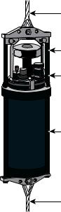
Acoustic-Doppler current meters are much simpler than the adcp. They transmit continuous beams of sound to measure current velocity close to the meter, not as a function of distance from the meter. They are placed on moorings and sometimes on a ctd. Instruments on moorings record velocity as a function of time for many days or months. The Aanderaa current meter (figure 10.19) in the figure is an example of this type. Instruments on ctds profile currents from the surface to the bottom at hydrographic stations.
10.10Important Concepts
1.Pressure distribution is almost precisely the hydrostatic pressure obtained by assuming the ocean is at rest. Pressure is therefore calculated very
10.10. IMPORTANT CONCEPTS |
181 |
Mooring Line
RCM Acoustic
Doppler Current Sensor
Optional Sensors: -Oxygen -Pressure -Temperature -Turbidity
Electronics and
Data Storage
Mooring Line
Figure 10.19 An example of a moored acoustic current meter, the rcm 9 produced by Aanderaa Instruments. Two components of horizontal velocity are measured by an acoustic system, and the directions are referenced to north using an internal Hall-e ect compass. The electronics, data recorder, and battery are in the pressure-resistant housing. Accuracy is
±0.15 cm/s and ±5◦. (Courtesy Aanderaa Instruments)
accurately from measurements of temperature and conductivity as a function of pressure using the equation of state of seawater. Hydrographic data give the relative, internal pressure field of the ocean.
2.Flow in the ocean is in almost exact geostrophic balance except for flow in the upper and lower boundary layers. Coriolis force almost exactly balances the horizontal pressure gradient.
3.Satellite altimetric observations of the oceanic topography give the surface geostrophic current. The calculation of topography requires an accurate geoid. If the geoid is not known, altimeters can measure the change in topography as a function of time, which gives the change in surface geostrophic currents.
4.Topex/Poseidon and Jason are the most accurate altimeter systems, and they can measure the topography or changes in topography with an accuracy of ±4 cm.
5.Hydrographic data are used to calculate the internal geostrophic currents in the ocean relative to known currents at some level. The level can be surface currents measured by altimetry or an assumed level of no motion at depths below 1–2 km.
6.Flow in the ocean that is independent of depth is called barotropic flow,
182 |
CHAPTER 10. GEOSTROPHIC CURRENTS |
flow that depends on depth is called baroclinic flow. Hydrographic data give only the baroclinic flow.
7.Geostrophic flow cannot change with time, so the flow in the ocean is not exactly geostrophic. The geostrophic method does not apply to flows at the equator where the Coriolis force vanishes.
8.Slopes of constant density or temperature surfaces seen in a cross-section of the ocean can be used to estimate the speed of flow through the section.
9.Lagrangian techniques measure the position of a parcel of water in the ocean. The position can be determined using surface drifters or subsurface floats, or chemical tracers such as tritium.
10.Eulerian techniques measure the velocity of flow past a point in the ocean. The velocity of the flow can be measured using moored current meters or acoustic velocity profilers on ships, ctds or moorings.
Chapter 11
Wind Driven Ocean
Circulation
What drives the ocean currents? At first, we might answer, the winds. But if we think more carefully about the question, we might not be so sure. We might notice, for example, that strong currents, such as the North Equatorial Countercurrents in the Atlantic and Pacific Ocean go upwind. Spanish navigators in the 16th century noticed strong northward currents along the Florida coast that seemed to be unrelated to the wind. How can this happen? And, why are strong currents found o shore of east coasts but not o shore of west coasts?
Answers to the questions can be found in a series of three remarkable papers published from 1947 to 1951. In the first, Harald Sverdrup (1947) showed that the circulation in the upper kilometer or so of the ocean is directly related to the curl of the wind stress if the Coriolis force varies with latitude. Henry Stommel (1948) showed that the circulation in oceanic gyres is asymmetric also because the Coriolis force varies with latitude. Finally, Walter Munk (1950) added eddy viscosity and calculated the circulation of the upper layers of the Pacific. Together the three oceanographers laid the foundations for a modern theory of ocean circulation.
11.1Sverdrup’s Theory of the Oceanic Circulation
While Sverdrup was analyzing observations of equatorial currents, he came upon (11.6) below relating the curl of the wind stress to mass transport within the upper ocean. To derive the relationship, Sverdrup assumed that the flow is stationary, that lateral friction and molecular viscosity are small, that non-linear terms such as u ∂u/∂x are small, and that turbulence near the sea surface can be described using a vertical eddy viscosity. He also assumed that the wind-driven circulation vanishes at some depth of no motion. With these assumptions, the horizontal components of the momentum equation from 8.9 and 8.12 become:
∂p |
= f ρ v + |
∂Txz |
(11.1a) |
|
∂x |
∂z |
|||
|
|
183
184 |
CHAPTER 11. WIND DRIVEN OCEAN CIRCULATION |
||||
|
|
∂p |
= −f ρ u + |
∂Tyz |
(11.1b) |
|
|
∂y |
∂z |
||
Sverdrup integrated these equations from the surface to a depth −D equal to or greater than the depth at which the horizontal pressure gradient becomes zero. He defined:
|
|
0 |
|
|
|
|
0 |
|
|
|
∂P |
|
ZD |
∂P |
|
ZD |
|
||||
|
= |
|
|
dz, |
|
= |
|
|
dz, |
(11.2a) |
∂x |
|
|
∂x |
∂y |
|
|
∂y |
|
||
|
|
− |
|
|
− |
|
||||
|
|
0 |
|
|
|
|
0 |
|
|
|
Mx ≡ |
ZD |
My ≡ |
ZD |
|
||||||
ρ u(z) dz, |
ρ v(z) dz, |
(11.2b) |
||||||||
|
|
− |
|
|
− |
|
||||
where Mx, My are the mass transports in the wind-driven layer extending down to an assumed depth of no motion.
The horizontal boundary condition at the sea surface is the wind stress. At depth −D the stress is zero because the currents go to zero:
Txz(0) = Tx |
Txz (−D) = 0 |
|
||
Tyz(0) = Ty |
Tyz (−D) = 0 |
(11.3) |
||
where Tx and Ty are the components of the wind stress. |
|
|||
Using these definitions and boundary conditions, (11.1) become: |
|
|||
|
∂P |
= f My + Tx |
(11.4a) |
|
|
|
|||
|
∂x |
|||
|
∂P |
= −f Mx + Ty |
(11.4b) |
|
|
|
|||
|
∂y |
|||
In a similar way, Sverdrup integrated the continuity equation (7.19) over the same vertical depth, assuming the vertical velocity at the surface and at depth −D are zero, to obtain:
∂Mx |
+ |
∂My |
= 0 |
(11.5) |
|
∂x |
∂y |
||||
|
|
|
Di erentiating (11.4a) with respect to y and (11.4b) with respect to x, subtracting, and using (11.5) gives:
β My = |
∂Ty |
− |
∂Tx |
|
∂x |
∂y |
|
||
β My = curlz (T ) |
(11.6) |
|||
where β ≡ ∂f /∂y is the rate of change of Coriolis parameter with latitude, and where curlz (T ) is the vertical component of the curl of the wind stress.
This is an important and fundamental result—the northward mass transport of wind driven currents is equal to the curl of the wind stress. Note that Sverdrup allowed f to vary with latitude. We will see later that this is essential.
11.1. SVERDRUP’S THEORY OF THE OCEANIC CIRCULATION |
185 |
|||||||||||||||||||||||||||||||||||||
|
|
|
|
|
|
|
|
|
|
|
|
|
|
|
|
|
|
|
|
|
|
|
|
|
|
|
|
|
|
|
|
|
|
|||||
|
|
|
|
|
|
|
|
|
|
|
|
|
|
|
|
|
|
|
|
|
|
|
|
|
|
|
|
|
|
|
|
|
|
|
|
|
|
|
30 o |
|
|
|
|
|
|
|
|
|
|
|
|
|
|
|
|
|
|
|
|
|
|
|
|
|
|
Streamlines of Mass |
|
|
|||||||||
|
|
|
-10 |
|
|
|
|
-5 |
|
|
|
|
|
|
|
|
|
|
|
|
|
|
|
|
|
|
Transport |
|
|
|
|
|
|
|||||
|
|
|
|
|
|
|
|
|
|
|
|
|
|
|
|
|
|
|
|
|
|
|
|
|
|
|
Boundaries of Counter |
|
|
|||||||||
|
|
|
|
|
|
|
|
|
|
|
|
|
|
|
|
|
|
|
|
|
|
|
|
|
|
|
|
|
||||||||||
|
|
|
|
|
|
|
|
|
|
|
|
|
|
|
|
|
|
|
|
|
|
|
|
|
|
|
|
|
|
Current |
|
|
|
|
|
|
||
20 o |
|
|
|
|
|
|
|
|
|
|
0 |
|
|
|
|
|
|
|
|
|
|
|
|
|
Values of stream function, Ψ, |
|
|
|||||||||||
|
|
|
|
|
|
|
|
|
|
|
|
|
|
|
|
|
|
|
|
given in units of 10 metric tons/sec |
|
|
||||||||||||||||
|
|
|
|
5 |
|
|
|
|
|
|
|
|
|
|
|
|
|
|
|
|
|
|
||||||||||||||||
|
|
|
|
|
|
|
|
|
|
|
|
|
|
|
|
|
|
|
|
|
|
|
|
|
|
|
|
|
|
|
|
|
|
|
|
|
||
|
|
15 |
|
10 |
|
|
|
|
|
|
|
|
|
|
|
|
|
|
|
|
|
|
|
|
|
|
|
|
|
|
|
|
|
|
|
|
|
|
10 o |
|
-15 |
10 |
|
|
|
|
|
|
|
|
|
|
|
|
|
|
|
|
|
|
|
|
|
|
|
|
|
|
|
|
|
|
|
|
|
|
|
|
|
|
|
|
|
|
|
|
|
|
|
|
|
|
|
|
|
|
|
|
|
|
|
|
|
|
|
|
|
|
|
|
|
|
||||
|
|
|
5 |
|
|
|
|
|
|
|
|
|
|
|
|
|
|
|
|
|
|
|
|
|
|
|
|
|
|
|
|
|
|
|
|
|||
|
|
|
|
|
|
|
|
|
|
|
|
|
|
|
|
|
|
|
|
|
|
|
|
|
|
|
|
|
|
|
|
|
|
|
|
|||
|
|
|
|
|
|
|
|
0 |
|
|
|
|
|
|
|
|
|
|
|
|
|
|
|
0 |
|
|
|
|
|
|
|
|
|
|
||||
|
|
15 |
|
-10 |
-5 |
|
|
|
|
|
|
|
|
|
|
|
|
|
|
|
|
|
|
|
|
|
|
|
|
|
|
|
||||||
|
|
|
|
|
|
|
|
|
|
|
|
|
|
|
|
|
|
|
|
|
|
|
|
|
|
|
|
|
|
|
|
|
|
|
||||
|
|
|
|
|
|
|
|
|
|
|
|
|
|
|
|
|
|
|
|
|
|
|
|
|
|
|
|
|
|
|
|
|
|
|
|
|
||
|
|
|
|
|
|
|
|
|
|
|
|
|
|
|
|
|
|
|
|
|
|
|
|
|
|
|
|
|
|
|
|
|
|
|
|
|
|
|
|
|
|
|
|
-20 |
|
|
|
|
|
|
|
|
|
|
|
|
|
|
|
|
|
|
|
|
|
|
|
|
|
|
|
|
|
|
|
|
|
0 o |
|
|
|
|
|
|
|
|
|
|
|
|
|
|
|
|
|
|
|
|
|
|
|
|
|
|
|
|
|
|
|
|
|
|
|
|
|
|
|
|
|
|
|
|
|
|
|
|
|
|
|
|
|
|
|
|
|
|
|
|
|
|
|
|
|
|
|
|
|
|
|
|
|
|
|
||
|
-15 |
|
-10 |
|
|
|
|
|
|
|
|
|
|
|
|
|
|
|
|
|
|
|
|
|
|
|
|
|
|
|
|
|
|
|
|
|
|
|
|
|
|
|
|
|
|
|
|
|
|
|
|
|
|
|
|
|
|
|
|
|
|
|
|
|
|
|
|
|
|
|
|
|
|
|
|
||
|
|
|
|
-5 |
|
|
|
|
|
|
|
|
|
|
|
|
|
|
|
|
|
|
|
|
|
|
|
|
|
|
|
|
|
|
|
|
||
|
|
|
|
|
|
|
0 |
|
|
|
|
|
|
|
|
|
|
|
|
|
|
|
|
0 |
|
|
|
|
|
|
|
|
|
|
||||
-10 o |
|
|
|
|
|
|
|
|
|
|
|
|
|
|
|
|
|
|
|
|
|
|
|
|
|
|
|
|
|
|
|
|
|
|
||||
|
|
|
|
|
|
|
|
|
|
|
|
|
|
|
|
|
|
|
|
|
|
|
|
|
|
|
|
|
|
|
|
|
|
|
|
|
|
|
|
|
|
|
|
|
|
|
|
|
|
|
|
|
|
|
|
|
|
|
|
|
|
|
|
|
|
|
|
|
|
|
|
|
|
|
|
|
|
|
|
25 |
|
|
|
|
|
|
|
|
|
|
|
15 |
|
|
|
|
|
|
10 |
|
|
|
5 |
|
|
|
|
|
|
|
|
|||||
|
|
|
|
|
|
|
|
|
|
|
|
|
|
|
|
|
|
|
|
|
|
|
|
|
|
|
|
|
|
|||||||||
|
|
|
|
20 |
|
|
|
|
|
|
|
|
|
|
|
|
|
|
|
|
|
|
|
|
|
|
|
|||||||||||
|
|
|
|
|
|
|
|
|
|
|
|
|
|
|
|
|
|
|
|
|
|
|
|
|
|
|
|
|||||||||||
-160 o |
-150 o |
|
-140 o |
|
|
|
-130 o |
|
-120 o |
|
-110 o |
-100 o |
|
|
|
-90 o |
-80 o |
|||||||||||||||||||||
|
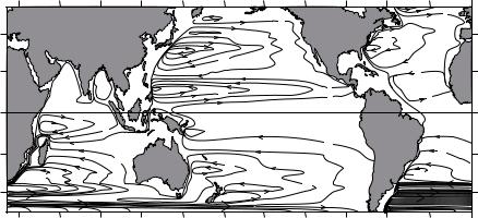
|
|
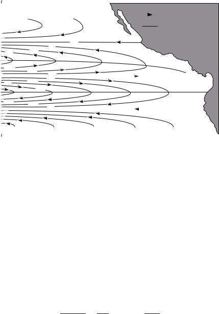
Figure 11.1 Streamlines of mass transport in the eastern Pacific calculated |
|
|
|
|
|
|
|||||||||||||||||||||||||||||
|
|
|
from Sverdrup’s theory using mean annual wind stress. After Reid (1948). |
|
|
|
|
|
|
|||||||||||||||||||||||||||||
|
We calculate β from |
|
|
|
|
|
|
|
|
|
|
|
|
|
|
|
|
|
|
|
|
|
|
|
|
|
|
|
|
|
|
|
||||||
|
|
|
|
|
|
|
|
|
|
|
β ≡ |
∂f |
= |
2 Ω cos ϕ |
|
|
|
|
|
|
|
|
|
(11.7) |
||||||||||||||
|
|
|
|
|
|
|
|
|
|
|
|
|
|
|
|
|
|
|
|
|
|
|
|
|
||||||||||||||
|
|
|
|
|
|
|
|
|
|
|
∂y |
|
|
R |
|
|
|
|
|
|
|
|
|
|||||||||||||||
where R is earth’s radius and ϕ is latitude.
Over much of the open ocean, especially in the tropics, the wind is zonal and ∂Ty/∂x is su ciently small that
My ≈ − |
1 |
|
∂Tx |
(11.8) |
β |
|
∂y |
Substituting (11.8) into (11.5), assuming β varies with latitude, Sverdrup ob-
tained: |
|
|
|
|
|
∂2Tx |
R |
|
|
|
∂Mx |
= − |
1 |
∂Tx |
tan ϕ + |
(11.9) |
|||
|
∂x |
2 Ω cos ϕ |
∂y |
∂y2 |
|||||
Sverdrup integrated this equation from a north-south eastern boundary at x = 0, assuming no flow into the boundary. This requires Mx = 0 at x = 0.
Then |
∂yx tan ϕ + |
∂2T |
x R |
(11.10) |
Mx = −2 Ω cos ϕ |
||||
x |
∂T |
|
|
∂y2
where x is the distance from the eastern boundary of the ocean basin, and brackets indicate zonal averages of the wind stress (figure 11.1).
To test his theory, Sverdrup compared transports calculated from known winds in the eastern tropical Pacific with transports calculated from hydrographic data collected by the Carnegie and Bushnell in October and November 1928, 1929, and 1939 between 34◦N and 10◦S and between 80◦W and 160◦W.
186 |
|
|
CHAPTER 11. WIND DRIVEN OCEAN CIRCULATION |
|||||||||||||||||||
|
|
|
Latitude |
|
|
|
|
|
Latitude |
|||||||||||||
|
|
|
25 |
|
|
|
|
|
|
|
|
25 |
|
|
|
|
|
|
|
|||
|
|
|
20 |
|
|
|
North Equatorial |
20 |
|
|
|
|
|
|
|
|||||||
|
|
|
|
|
|
|
Current |
|
|
|
|
|
|
|
||||||||
|
|
|
|
|
|
|
|
|
|
|
|
|
|
|
|
|
|
|
||||
|
|
|
15 |
|
|
|
|
|
|
|
|
15 |
|
|
|
|
|
|
|
|||
|
|
|
|
|
|
|
|
|
|
|
|
|
|
|
|
|
|
|||||
|
|
|
|
|
|
|
|
|
|
|
|
|
|
|
|
|
|
|
|
|||
|
|
|
10 |
|
|
|
|
|
|
|
|
10 |
|
|
|
|
|
|
|
|||
|
|
|
|
|
|
|
|
North Equatorial |
|
|
|
|
|
|
|
|
|
|
||||
|
|
|
5 |
|
|
|
Counter Current |
5 |
|
|
|
|
|
|
|
|||||||
|
|
|
|
|
|
|
|
|
|
|
|
|
|
|
|
|
|
|
|
|
|
Mx |
|
|
|
|
|
|
|
|
My |
|
|
|
|
|
|
|
|
|
|
|
|||
|
|
|
|
|
|
|
|
|
|
|
|
|||||||||||
-7 -5 |
-3 -1 1 3 5 |
-50 -30 |
-10 10 30 50 70 |
|||||||||||||||||||
Southward |
-5 |
|
|
|
Northward |
|
Westward |
-5 |
|
|
|
Eastward |
||||||||||
|
|
|
|
|
|
South Equatorial |
|
|
|
|
|
|
|
|||||||||
|
|
|
|
|
|
|
|
|
|
|
|
|
|
|
|
|
|
|||||
|
|
|
|
|
|
|
|
|
Current |
|
|
|
|
|
|
|
|
|
|
|||
|
|
|
-10 |
|
|
|
|
|
|
|
|
-10 |
|
|
|
|
|
|
|
|||
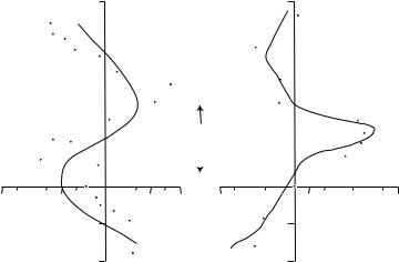
Figure 11.2 Mass transport in the eastern Pacific calculated from Sverdrup’s theory using observed winds with 11.8 and 11.10 (solid lines) and pressure calculated from hydrographic data from ships with 11.4 (dots). Transport is in tons per second through a section one meter wide extending from the sea surface to a depth of one kilometer. Note the di erence in scale between My and Mx. After Reid (1948).
The hydrographic data were used to compute P by integrating from a depth of D = −1000 m. The comparison, figures 11.2, showed not only that the transports can be accurately calculated from the wind, but also that the theory predicts wind-driven currents going upwind.
Comments on Sverdrup’s Solutions
1.Sverdrup assumed i) The internal flow in the ocean is geostrophic; ii) there is a uniform depth of no motion; and iii) Ekman’s transport is correct. I examined Ekman’s theory in Chapter 9, and the geostrophic balance in Chapter 10. We know little about the depth of no motion in the tropical Pacific.
2.The solutions are limited to the east side of the ocean because Mx grows with x. The result comes from neglecting friction which would eventually balance the wind-driven flow. Nevertheless, Sverdrup solutions have been used for describing the global system of surface currents. The solutions are applied throughout each basin all the way to the western limit of the basin. There, conservation of mass is forced by including north-south currents confined to a thin, horizontal boundary layer (figure 11.3).
3.Only one boundary condition can be satisfied, no flow through the eastern boundary. More complete descriptions of the flow require more complete equations.
4.The solutions do not give the vertical distribution of the current.
5.Results were based on data from two cruises plus average wind data assuming a steady state. Later calculations by Leetmaa, McCreary, and
11.1. SVERDRUP’S THEORY OF THE OCEANIC CIRCULATION |
187 |
||
|
|
0 |
|
40 o |
|
|
|
|
20 |
|
|
20 o |
|
|
|
|
20 |
0 |
|
|
|
|
|
0 o |
|
|
|
-20 o |
|
20 |
|
|
30 |
|
|
-40 o |
|
|
|
30 o 60o |
90o 120o 150 o 180 o -150 o -120 o -90 o -60 o -30 o |
0 o |
|
Figure 11.3 Depth-integrated Sverdrup transport applied globally using the wind stress from Hellerman and Rosenstein (1983). Contour interval is 10 Sverdrups. After Tomczak and Godfrey (1994: 46).
Moore (1981) using more recent wind data produces solutions with seasonal variability that agrees well with observations provided the level of no motion is at 500 m. If another depth were chosen, the results are not as good.
6.Wunsch (1996: §2.2.3) after carefully examining the evidence for a Sverdrup balance in the ocean concluded we do not have su cient information to test the theory. He writes
The purpose of this extended discussion has not been to disapprove the validity of Sverdrup balance. Rather, it was to emphasize the gap commonly existing in oceanography between a plausible and attractive theoretical idea and the ability to demonstrate its quantitative applicability to actual oceanic flow fields.—Wunsch (1996).
Wunsch, however, notes
Sverdrup’s relationship is so central to theories of the ocean circulation that almost all discussions assume it to be valid without any comment at all and proceed to calculate its consequences for higherorder dynamics. . . it is di cult to overestimate the importance of Sverdrup balance.—Wunsch (1996).
But the gap is shrinking. Measurements of mean stress in the equatorial Pacific (Yu and McPhaden, 1999) show that the flow there is in Sverdrup balance.
Stream Lines, Path Lines, and the Stream Function Before discussing more about the ocean’s wind-driven circulation, we need to introduce the concept of stream lines and the stream function (see Kundu, 1990: 51 & 66).
At each instant in time, we can represent a flow field by a vector velocity at each point in space. The instantaneous curves that are everywhere tangent to
188 |
CHAPTER 11. WIND DRIVEN OCEAN CIRCULATION |
y 
x + d x
-u dy
xv dx
ψ
+
d ψ
ψ
x
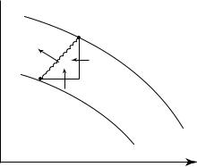
Figure 11.4 Volume transport between stream lines in a two-dimensional, steady flow. After Kundu (1990: 68).
the direction of the vectors are called the stream lines of the flow. If the flow is unsteady, the pattern of stream lines change with time.
The trajectory of a fluid particle, the path followed by a Lagrangian drifter, is called the path line in fluid mechanics. The path line is the same as the stream line for steady flow, and they are di erent for an unsteady flow.
We can simplify the description of two-dimensional, incompressible flows by using the stream function ψ defined by:
u ≡ |
∂ψ |
, |
v ≡ − |
∂ψ |
, |
(11.11) |
|
|
|||||
∂y |
∂x |
The stream function is often used because it is a scalar from which the vector velocity field can be calculated. This leads to simpler equations for some flows.
Stream functions are also useful for visualizing the flow. At each instant, the flow is parallel to lines of constant ψ. Thus if the flow is steady, the lines of constant stream function are the paths followed by water parcels.
The volume rate of flow between any two stream lines of a steady flow is dψ, and the volume rate of flow between two stream lines ψ1 and ψ2 is equal to ψ1 − ψ2. To see this, consider an arbitrary line dx = (dx, dy) between two stream lines (figure 11.4). The volume rate of flow between the stream lines is:
|
∂ψ |
∂ψ |
|
||
v dx + (−u) dy = − |
|
dx − |
|
dy = −dψ |
(11.12) |
∂x |
∂y |
||||
and the volume rate of flow between the two stream lines is numerically equal to the di erence in their values of ψ.
Now, lets apply the concepts to satellite-altimeter maps of the oceanic to-
pography. In §10.3 I wrote (10.10) |
|
|
g ∂ζ |
|
||||
us = − |
|
|||||||
|
|
|
|
|
|
|||
f |
∂y |
|
||||||
vs = |
g |
|
∂ζ |
(11.13) |
||||
|
|
|
|
|
||||
f |
|
∂x |
||||||