Numerical Models

Discretization is essential for computer implementation and cannot be dispensed with. The essence of the di culty is that the dynamics of discrete systems is only loosely related to that of continuous systems—indeed the dynamics of discrete systems is far richer than that of their continuous counterparts—and the approximations involved can create spurious solutions.

Calculations of turbulence are di cult. Numerical models provide information only at grid points of the model. They provide no information about the flow between the points. Yet, the ocean is turbulent, and any oceanic model capable of resolving the turbulence needs grid points spaced millimeters apart, with time steps of milliseconds.

Practical ocean models have grid points spaced tens to hundreds of kilometers apart in the horizontal, and tens to hundreds of meters apart in the vertical. This means that turbulence cannot be calculated directly, and the influence of turbulence must be parameterized. Holloway (1994) states the problem succinctly:

Ocean models retain fewer degrees of freedom than the actual ocean (by about 20 orders of magnitude). We compensate by applying ‘eddyviscous goo’ to squash motion at all but the smallest retained scales. (We also use non-conservative numerics.) This is analogous to placing a partition in a box to prevent gas molecules from invading another region of the box. Our oceanic models cannot invade most of the real oceanic degrees of freedom simply because the models do not include them.

Given that we cannot do things ‘right’, is it better to do nothing? That is not an option. ‘Nothing’ means applying viscous goo and wishing for the ever bigger computer. Can we do better? For example, can we guess a higher entropy configuration toward which the eddies tend to drive the ocean (that tendency to compete with the imposed forcing and dissipation)?

By “degrees of freedom” Holloway means all possible motions from the smallest waves and turbulence to the largest currents. Let’s do a calculation. We know that the ocean is turbulent with eddies as small as a few millimeters. To completely describe the ocean we need a model with grid points spaced 1 mm apart and time steps of about 1 ms. The model must therefore have 360◦× 180◦× (111 km/degree)2 ×1012 (mm/km)2× 3 km ×106 (mm/km) = 2.4 ×1027 data points for a 3 km deep ocean covering the globe. The global Parallel Ocean Program Model described in the next section has 2.2 × 107 points. So we need 1020 times more points to describe the real ocean. These are the missing 1020 degrees of freedom.

Practical models must be simpler than the real ocean. Models of the ocean must run on available computers. This means oceanographers further simplify their models. We use the hydrostatic and Boussinesq approximations, and we often use equations integrated in the vertical, the shallow-water equations (Haidvogel and Beckmann, 1999: 37). We do this because we cannot yet run the most detailed models of oceanic circulation for thousands of years to understand the role of the ocean in climate.

Numerical code has errors. Do you know of any software without bugs? Numerical models use many subroutines each with many lines of code which are converted into instructions understood by processors using other software called a compiler. Eliminating all software errors is impossible. With careful testing, the output may be correct, but the accuracy cannot be guaranteed. Plus, numerical calculations cannot be more accurate than the accuracy of the floating-point numbers and integers used by the computer. Round-o errors cannot be ignored. Lawrence et al (1999), examining the output of an atmospheric numerical model found an error in the code produced by the fortran-90 compiler used on the cray Research supercomputer used to run the code. They also found round-o errors in the concentration of tracers calculated from the model. Both errors produced important errors in the output of the model.

Most models are not well verified or validated (Post & Votta, 2005). Yet, without adequate verification and validation, output from numerical models is not credible.

Summary Despite these many sources of error, most are small in practice. Numerical models of the ocean are giving the most detailed and complete views of the circulation available to oceanographers. Some of the simulations contain unprecedented details of the flow. I included the words of warning not to lead you to believe the models are wrong, but to lead you to accept the output with a grain of salt.

15.2Numerical Models in Oceanography

Numerical models are very widely used for many purposes in oceanography. For our purpose we can divide models into two classes:

Mechanistic models are simplified models used for studying processes. Because the models are simplified, the output is easier to interpret than output from more complex models. Many di erent types of simplified models have been developed, including models for describing planetary waves, the interaction of the flow with sea-floor features, or the response of the upper ocean to the wind. These are perhaps the most useful of all models because they provide insight into the physical mechanisms influencing the ocean. The development and use of mechanistic models is, unfortunately, beyond the scope of this book.

Simulation models are used for calculating realistic circulation of oceanic regions. The models are often very complex because all important processes are included, and the output is di cult to interpret.

The first simulation model was developed by Kirk Bryan and Michael Cox (Bryan, 1969) at the Geophysical Fluid Dynamics laboratory in Princeton. They calculated the 3-dimensional flow in the ocean using the continuity and momentum equation with the hydrostatic and Boussinesq approximations and a simple equation of state. Such models are called primitive equation models because they use the basic, or primitive form of the equations of motion. The equation of state allows the model to calculate changes in density due to fluxes of heat and water through the surface, so the model includes thermodynamic processes.

The Bryan-Cox model used large horizontal and vertical viscosity and di u- sion to eliminate turbulent eddies having diameters smaller about 500 km, which is a few grid points in the model. It had complex coastlines, smoothed sea-floor features, and a rigid lid. The rigid lid was needed to eliminate ocean-surface waves, such as tides and tsunamis, that move far too fast for the coarse time steps used by all simulation models. The rigid lid had, however, disadvantages. Islands substantially slowed the computation, and the sea-floor features were smoothed to eliminate steep gradients.

The first simulation model was regional. It was quickly followed by a global model (Cox, 1975) with a horizontal resolution of 2◦ and with 12 levels in the vertical. The model ran far too slowly even on the fastest computers of the day, but it laid the foundation for more recent models. The coarse spatial resolution required that the model have large values for viscosity, and even regional models were too viscous to have realistic western boundary currents or mesoscale eddies.

Since those times, the goal has been to produce models with ever finer resolution, more realistic modeling of physical processes, and better numerical schemes. Computer technology is changing rapidly, and models are evolving rapidly. The output from the most recent models of the north Atlantic, which have resolution of 0.03◦ look very much like the real ocean. Models of other areas show previously unknown currents near Australia and in the south Atlantic.

Ocean and Atmosphere Models use very di erent spacing of grid points. As a result, ocean modeling lags about a decade behind atmosphere modeling. Dominant ocean eddies are 1/30 the size of dominant atmosphere eddies (storms). But, ocean features evolve at a rate that is 1/30 the rate in the atmosphere. Thus ocean models running for say one year have (30 × 30) more horizontal grid points than the atmosphere, but they have 1/30 the number of time steps. Both have about the same number of grid points in the vertical. As a result, ocean models run 30 times slower than atmosphere models of the same complexity.

15.3Global Ocean Models

Several types of global models are widely used in oceanography. Most have grid points about one tenth of a degree apart, which is su cient to resolve mesoscale eddies, such as those seen in figures 11.10, 11.11, and 15.2, that have a diameter larger than two to three times the distance between grid points. Vertical resolution is typically around 30 vertical levels. Models include: i) realistic coasts and bottom features; ii) heat and water fluxes though the surface; iii) eddy dynamics; and iv) the meridional-overturning circulation. Many assimilate satellite and float data using techniques described in §15.5. The models range in complexity from those that can run on desktop workstations to those that require the world’s fastest computers.

All models must be be run to calculate one to two decades of variability before they can be used to simulate the ocean. This is called spin-up. Spin-up is needed because initial conditions for density, fluxes of momentum and heat through the sea-surface, and the equations of motion are not all consistent.

Models are started from rest with values of density from the Levitus (1982) atlas and integrated for a decade using mean-annual wind stress, heat fluxes, and water flux. The model may be integrated for several more years using monthly wind stress, heat fluxes, and water fluxes.

The Bryan-Cox models evolved into several widely used models which are providing impressive views of the global ocean circulation.

Geophysical Fluid Dynamics Laboratory Modular Ocean Model MOM consistsof a large set of modules that can be configured to run on many di erent computersto model many di erent aspects of the circulation. The source code is open and free, and it is in the public domain. The model is widely use for climate studies and for studying the ocean’s circulation over a wide range of space and time scales (Pacanowski and Gri es, 1999).

Because mom is used to investigate processes which cover a wide range of time and space scales, the code and manual are lengthy. However, it is far from necessary for the typical ocean modeler to become acquainted with all of its aspects. Indeed, mom can be likened to a growing city with many di erent neighborhoods. Some of the neighborhoods communicate with one another, some are mutually incompatible, and others are basically independent. This diversity is quite a challenge to coordinate and support. Indeed, over the years certain “neighborhoods” have been jettisoned or greatly renovated for various reasons.—Pacanowski and Gri es.

The model uses the momentum equations, equation of state, and the hydrostatic and Boussinesq approximations. Subgrid-scale motions are reduced by use of eddy viscosity. Version 4 of the model has improved numerical schemes, a free surface, realistic bottom features, and many types of mixing including horizontal mixing along surfaces of constant density. Plus, it can be coupled to atmospheric models.

Parallel Ocean Program Model produced by Smith and colleagues at Los Alamos National Laboratory (Maltrud et al, 1998) is another widely used model growing out of the original Bryan-Cox code. The model includes improved numerical algorithms, realistic coasts, islands, and unsmoothed bottom features. It has model has 1280 ×896 equally spaced grid points on a Mercator projection extending from 77◦S to 77◦N, and 20 levels in the vertical. Thus it has 2.2 ×107 points giving a resolution of 0.28◦ × 0.28◦ cos θ, which varies from 0.28◦ (31.25 km) at the equator to 0.06◦ (6.5 km) at the highest latitudes. The average resolution is about 0.2◦. The model was is forced by ecmwf wind stress and surface heat and water fluxes (Barnier et al, 1995).

Hybrid Coordinate Ocean Model hycom All the models just described use x, y, z coordinates. Such a coordinate system has both advantages and disadvantages. It can have high resolution in the surface mixed layer and in shallower regions. But it is less useful in the interior of the ocean. Below the mixed layer, mixing in the ocean is easy along surfaces of constant density, and di cult across such surfaces. A more natural coordinate system in the interior of the ocean uses x, y, ρ, where ρ is density. Such a model is called an isopycnal

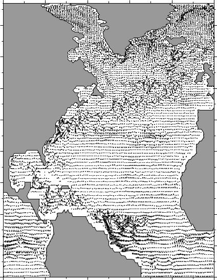
Figure 15.1 Near-surface geostrophic currents on October 1, 1995 calculated by the Parallel Ocean Program numerical model developed at the Los Alamos National Laboratory. The length of the vector is the mean speed in the upper 50 m of the ocean. The direction is the mean direction of the current. From Richard Smith, Los Alamos National Laboratory.

model . Essentially, ρ(z) is replaced with z(ρ). Because isopycnal surfaces are surfaces of constant density, horizontal mixing is always on constant-density surfaces in this model.

The Hybrid Coordinate Ocean Model hycom model uses di erent vertical coordinates in di erent regions of the ocean, combining the best aspects of z- coordinate model and isopycnal-coordinate model (Bleck, 2002). The hybrid model has evolved from the Miami Isopycnic-Coordinate Ocean Model (fig-

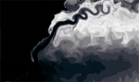
Figure 15.2 Output of Bleck’s Miami Isopycnal Coordinate Ocean Model micom. It is a high-resolution model of the Atlantic showing the Gulf Stream, its variability, and the circulation of the north Atlantic. From Bleck.

ure 15.2). It is a primitive-equation model driven by wind stress and heat fluxes. It has realistic mixed layer and improved horizontal and vertical mixing schemes that include the influences of internal waves, shear instability, and double-di usion (see §8.5). The model results from collaborative work among investigators at many oceanographic laboratories.

Regional Oceanic Modeling System roms is a regional model that can be imbedded in models of much larger regions. It is widely used for studying coastal current systems closely tied to flow further o shore, for example, the California Current. roms is a hydrostatic, primitive equation, terrain-following model using stretched vertical coordinates, driven by surface fluxes of momentum, heat, and water. It has improved surface and bottom boundary layers (Shchepetkin and McWilliams, 2004).

Climate models are used for studies of large-scale hydrographic structure, climate dynamics, and water-mass formation. These models are the same as the eddy-admitting, primitive equation models I have just described except the horizontal resolution is much coarser because they must simulate ocean processes for decades or centuries. As a result, they must have high dissipation for numerical stability, and they cannot simulate mesoscale eddies. Typical horizontal resolutions are 2◦ to 4◦. The models tend, however, to have high vertical resolution necessary for describing the deep circulation important for climate.