6.2. DEFINITION OF TEMPERATURE

6.2Definition of Temperature

Many physical processes depend on temperature. A few can be used to define absolute temperature T . The unit of T is the kelvin, which has the symbol K. The fundamental processes used for defining an absolute temperature scale over the range of temperatures found in the ocean include (Soulen and Fogle, 1997): 1) the gas laws relating pressure to temperature of an ideal gas with corrections for the density of the gas; and 2) the voltage noise of a resistance R.

The measurement of temperature using an absolute scale is di cult and the measurement is usually made by national standards laboratories. The absolute measurements are used to define a practical temperature scale based on the temperature of a few fixed points and interpolating devices which are calibrated at the fixed points.

For temperatures commonly found in the ocean, the interpolating device is a platinum-resistance thermometer. It consists of a loosely wound, strain-free, pure platinum wire whose resistance is a function of temperature. It is calibrated at fixed points between the triple point of equilibrium hydrogen at 13.8033 K and the freezing point of silver at 961.78 K, including the triple point of water at 0.060◦C, the melting point of Gallium at 29.7646◦C, and the freezing point of Indium at 156.5985◦C (Preston-Thomas, 1990). The triple point of water is the temperature at which ice, water, and water vapor are in equilibrium. The temperature scale in kelvin T is related to the temperature scale in degrees Celsius t[◦C] by:

The practical temperature scale was revised in 1887, 1927, 1948, 1968, and 1990 as more accurate determinations of absolute temperature became accepted. The most recent scale is the International Temperature Scale of 1990 (its-90). It di ers slightly from the International Practical Temperature Scale of 1968 ipts-68. At 0◦C they are the same, and above 0◦C its-90 is slightly cooler. t90 − t68 = −0.002 at 10◦C, −0.005 at 20◦C, −0.007 at 30◦C and −0.010 at 40◦C.

Notice that while oceanographers use thermometers calibrated with an accuracy of a millidegree, which is 0.001◦C, the temperature scale itself has uncertainties of a few millidegrees.

6.3 Geographical Distribution of Surface Temperature and Salinity

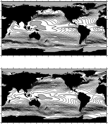
The distribution of temperature at the sea surface tends to be zonal, that is, it is independent of longitude (figure 6.2). Warmest water is near the equator, coldest water is near the poles. The deviations from zonal are small. Equatorward of 40◦, cooler waters tend to be on the eastern side of the basin. North of this latitude, cooler waters tend to be on the western side.

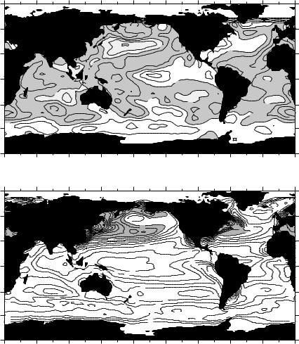
The anomalies of sea-surface temperature, the deviation from a long term average, are small, less than 1.5◦C (Harrison and Larkin, 1998) except in the equatorial Pacific where the deviations can be 3◦C (figure 6.3: top).

The annual range of surface temperature is highest at mid-latitudes, especially on the western side of the ocean (figure 6.3: bottom). In the west, cold air

Average Sea-Surface Temperature for July

Figure 6.2 Mean sea-surface temperature calculated from the optimal interpolation technique (Reynolds and Smith, 1995) using ship reports and avhrr measurements of temperature. Contour interval is 1◦C with heavy contours every 5◦C. Shaded areas exceed 29◦C.

blows o the continents in winter and cools the ocean. The cooling dominates the heat budget. In the tropics the temperature range is mostly less than 2◦C.

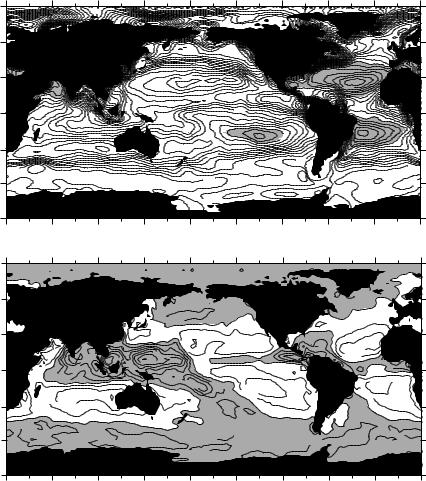
The distribution of sea-surface salinity also tends to be zonal. The saltiest waters are at mid-latitudes where evaporation is high. Less salty waters are near the equator where rain freshens the surface, and at high latitudes where melted sea ice freshens the surface (figure 6.4). The zonal (east-west) average of salinity shows a close correlation between salinity and evaporation minus precipitation plus river input (figure 6.5).

Because many large rivers drain into the Atlantic and the Arctic Sea, why is the Atlantic saltier than the Pacific? Broecker (1997) showed that 0.32 Sv of

the water evaporated from the Atlantic does not fall as rain on land. Instead, it is carried by winds into the Pacific (figure 6.6). Broecker points out that the quantity is small, equivalent to a little more than the flow in the Amazon River, but “were this flux not compensated by an exchange of more salty Atlantic waters for less salty Pacific waters, the salinity of the entire Atlantic would rise about 1 gram per liter per millennium.”

Mean Temperature and Salinity of the Ocean The mean temperature of the

Optimal Interpolation Monthly SST Anomalies for Jan. 1996

Figure 6.3 Top: Sea-surface temperature anomaly for January 1996 relative to mean temperature shown in figure 6.2 using data published by Reynolds and Smith (1995) in the Climate Diagnostics Bulletin for February 1995. Contour interval is 1◦C. Shaded areas are positive. Bottom:Annual range of sea-surface temperature in ◦C calculated from the Reynolds and Smith (1995) mean sea-surface temperature data set. Contour interval is 1◦C with heavy contours at 4◦C and 8◦C. Shaded areas exceed 8◦C.

Annual Mean Sea Surface Salinity

Figure 6.4 Top: Mean sea-surface salinity. Contour interval is 0.25. Shaded areas exceed a salinity of 36. From Levitus (1982). Bottom: Precipitation minus evaporation in meters per year calculated from global rainfall by the Global Precipitation Climatology Project and latent heat flux calculated by the Data Assimilation O ce, both at nasa’s Goddard Space Flight Center. Precipitation exceeds evaporation in the shaded regions, contour interval is 0.5 m.

ocean’s waters is: t = 3.5◦C. The mean salinity is S = 34.7. The distribution about the mean is small: 50% of the water is in the range:

1.3◦C < t < 3.8◦C

34.6 < S < 34.8