10.5An Example Using Hydrographic Data

Let’s now consider a specific numerical calculation of geostrophic velocity using generally accepted procedures from Processing of Oceanographic Station Data (jpots Editorial Panel, 1991). The book has worked examples using hydrographic data collected by the r/v Endeavor in the north Atlantic. Data were collected on Cruise 88 along 71◦W across the Gulf Stream south of Cape Cod, Massachusetts at stations 61 and 64. Station 61 is on the Sargasso Sea side of the Gulf Stream in water 4260 m deep. Station 64 is north of the Gulf Stream in water 3892 m deep. The measurements were made by a Conductivity- Temperature-Depth-Oxygen Profiler, Mark III CTD/02, made by Neil Brown Instruments Systems.

The ctd sampled temperature, salinity, and pressure 22 times per second, and the digital data were averaged over 2 dbar intervals as the ctd was lowered in the water. Data were tabulated at 2 dbar pressure intervals centered on odd values of pressure because the first observation is at the surface, and the first averaging interval extends to 2 dbar, and the center of the first interval is at 1 dbar. Data were further smoothed with a binomial filter and linearly interpolated to standard levels reported in the first three columns of tables 10.2 and 10.3. All processing was done by computer.

δ(S, t, p) in the fifth column of tables 10.2 and 10.3 is calculated from the values of t, S, p in the layer. < δ > is the average value of specific volume anomaly for the layer between standard pressure levels. It is the average of the values of δ(S, t, p) at the top and bottom of the layer (cf. the mean-value theorem of calculus). The last column (10−5ΔΦ) is the product of the average specific volume anomaly of the layer times the thickness of the layer in decibars. Therefore, the last column is the geopotential anomaly ΔΦ calculated by integrating (10.16) between P1 at the bottom of each layer and P2 at the top of each layer.

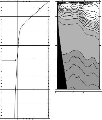
The distance between the stations is L = 110, 935 m; the average Coriolis parameter is f = 0.88104×10−4; and the denominator in (10.17) is 0.10231 s/m. This was used to calculate the geostrophic currents relative to 2000 decibars reported in table 10.4 and plotted in figure 10.8.

Notice that there are no Ekman currents in figure 10.8. Ekman currents are not geostrophic, so they don’t contribute directly to the topography. They contribute only indirectly through Ekman pumping (see figure 12.7).

10.6Comments on Geostrophic Currents

Now that we know how to calculate geostrophic currents from hydrographic data, let’s consider some of the limitations of the theory and techniques.

Converting Relative Velocity to Velocity Hydrographic data give geostrophic currents relative to geostrophic currents at some reference level. How can we convert the relative geostrophic velocities to velocities relative to the earth?

1.Assume a Level of no Motion: Traditionally, oceanographers assume there is a level of no motion, sometimes called a reference surface, roughly 2,000 m below the surface. This is the assumption used to derive the currents in table 10.4. Currents are assumed to be zero at this depth, and relative currents are integrated up to the surface and down to the bottom to

obtain current velocity as a function of depth. There is some experimental evidence that such a level exists on average for mean currents (see for example, Defant, 1961: 492).

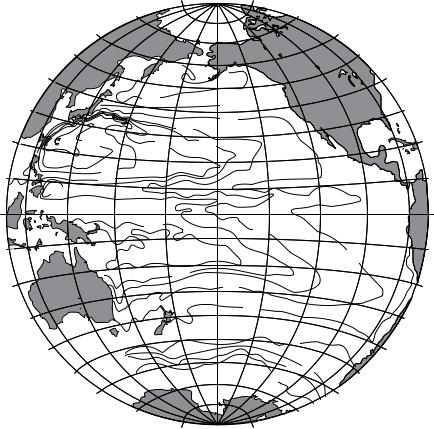
Defant recommends choosing a reference level where the current shear in the vertical is smallest. This is usually near 2 km. This leads to useful maps of surface currents because surface currents tend to be faster than deeper currents. Figure 10.9 shows the geopotential anomaly and surface currents in the Pacific relative to the 1,000 dbar pressure level.

2. Use known currents: The known currents could be measured by current

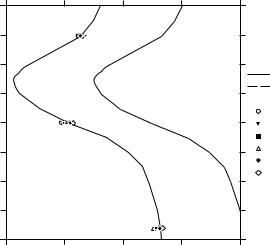
meters or by satellite altimetry. Problems arise if the currents are not measured at the same time as the hydrographic data. For example, the hydrographic data may have been collected over a period of months to decades, while the currents may have been measured over a period of only a few months. Hence, the hydrography may not be consistent with the current measurements. Sometimes currents and hydrographic data are measured at nearly the same time (figure 10.10). In this example, currents were measured continuously by moored current meters (points) in a deep western boundary current and calculated from ctd data taken just after the current meters were deployed and just before they were

Geopotential anomaly integrated from 2000 dbar level. Velocity is calculated from (10.17)

recovered (smooth curves). The solid line is the current assuming a level of no motion at 2,000 m, the dotted line is the current adjusted using the current meter observations smoothed for various intervals before or after the ctd casts.

3.Use Conservation Equations: Lines of hydrographic stations across a strait or an ocean basin may be used with conservation of mass and salt to calculate currents. This is an example of an inverse problem (Wunsch, 1996 describes the application of inverse methods in oceanography). See Mercier et al. (2003) for a description of how they determined the cir-

Figure 10.8 Left Relative current as a function of depth calculated from hydrographic data collected by the Endeavor cruise south of Cape Cod in August 1982. The Gulf Stream is the fast current shallower than 1000 decibars. The assumed depth of no motion is at 2000 decibars. Right Cross section of potential density σθ across the Gulf Stream along 63.66◦W calculated from ctd data collected from Endeavor on 25–28 April 1986. The Gulf Stream is centered on the steeply sloping contours shallower than 1000m between 40◦ and 41◦. Notice that the vertical scale is 425 times the horizontal scale. (Data contoured by Lynn Talley, Scripps Institution of Oceanography).

culation in the upper layers of the eastern basins of the south Atlantic using hydrographic data from the World Ocean Circulation Experiment and direct measurements of current in a box model constrained by inverse theory.

Disadvantage of Calculating Currents from Hydrographic Data Currents calculated from hydrographic data have been used to make maps of ocean currents since the early 20th century. Nevertheless, it is important to review the limitations of the technique.

1.Hydrographic data can be used to calculate only the current relative to a current at another level.

Figure 10.10 Current meter measurements can be used with ctd measurements to determine current as a function of depth avoiding the need for assuming a depth of no motion. Solid line: profile assuming a depth of no motion at 2000 decibars. Dashed line: profile adjusted to agree with currents measured by current meters 1–7 days before the ctd measurements. (Plots from Tom Whitworth, Texas A&M University)

acceleration of the flow. Acceleration dominates if the horizontal dimensions are less than roughly 50 km and times are less than a few days. Acceleration is negligible, but not zero, over longer times and distances.

2.The geostrophic balance does not apply within about 2◦ of the equator where the Coriolis force goes to zero because sin ϕ → 0.

3.The geostrophic balance ignores the influence of friction.

Accuracy Strub et al. (1997) showed that currents calculated from satellite altimeter measurements of sea-surface slope have an accuracy of ±3–5 cm/s. Uchida, Imawaki, and Hu (1998) compared currents measured by drifters in the Kuroshio with currents calculated from satellite altimeter data assuming geostrophic balance. Using slopes over distances of 12.5 km, they found the di erence between the two measurements was ±16 cm/s for currents up to 150 cm/s, or about 10%. Johns, Watts, and Rossby (1989) measured the velocity of the Gulf Stream northeast of Cape Hatteras and compared the measurements with velocity calculated from hydrographic data assuming geostrophic balance. They found that the measured velocity in the core of the stream, at depths less than 500 m, was 10–25 cm/s faster than the velocity calculated from the geostrophic equations using measured velocities at a depth of 2000 m. The maximum velocity in the core was greater than 150 cm/s, so the error was ≈ 10%. When they added the influence of the curvature of the Gulf Stream, which adds an acceleration term to the geostrophic equations, the di erence in the calculated and observed velocity dropped to less than 5–10 cm/s (≈ 5%).