Global Precipitation for 1995

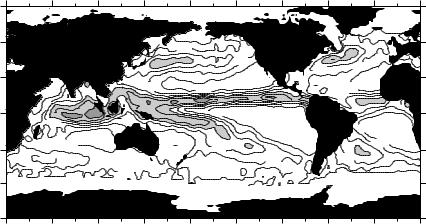
Figure 5.5 Rainfall in m/year calculated from data compiled by the Global Precipitation Climatology Project at nasa’s Goddard Space Flight Center using data from rain gauges, infrared radiometers on geosynchronous meteorological satellites, and the ssm/i. Contour interval is 0.5 m/yr, light shaded areas exceed 2 m/yr, heavy shaded areas exceed 3 m/yr.

The fluxes are not calculated from satellite data because satellite instruments are not very sensitive to water vapor close to the sea. Perhaps the best fluxes are those calculated from numerical weather models.

Sensible Heat Flux Sensible heat flux is calculated from observations of airsea temperature di erence and wind speed made from ships, or by numerical weather models. Sensible fluxes are small almost everywhere except o shore of the east coasts of continents in winter when cold, Arctic air masses extract heat from warm, western, boundary currents. In these areas, numerical models give perhaps the best values of the fluxes. Historical ship report give the long-term mean values of the fluxes.

5.5Global Data Sets for Fluxes

Ship and satellite data have been processed to produce global maps of fluxes. Ship measurements made over the past 150 years yield maps of the long-term mean values of the fluxes, especially in the northern hemisphere. Ship data, however, are sparse in time and space, and they are being replaced more and more by fluxes calculated by numerical weather models and by satellite data.

The most useful maps are those made by combining level 3 and 4 satellite data sets with observations from ships, using numerical weather models. Let’s look first at the sources of data, then at a few of the more widely used data sets.

International Comprehensive Ocean-Atmosphere Data Set Data collected by observers on ships are the richest source of marine information. Slutz et al. (1985) describing their e orts to collect, edit, and publish all marine observations write:

Since 1854, ships of many countries have been taking regular observations of local weather, sea surface temperature, and many other characteristics near the boundary between the ocean and the atmosphere. The observations by one such ship-of-opportunity at one time and place, usually incidental to its voyage, make up a marine report. In later years fixed research vessels, buoys, and other devices have contributed data. Marine reports have been collected, often in machine-readable form, by various agencies and countries. That vast collection of data, spanning the ocean from the mid-nineteenth century to date, is the historical oceanatmosphere record.

These marine reports have been edited and published as the International Comprehensive Ocean-Atmosphere Data Set icoads (Woodru et al. 1987) available through the National Oceanic and Atmospheric Administration.

The icoads release 2.3 includes 213 million reports of marine surface conditions collected from 1784–2005 by buoys, other platform types, and by observers on merchant ships. The data set include fully quality-controlled (trimmed) reports and summaries. Each unique report contains 22 observed and derived variables, as well as flags indicating which observations were statistically trimmed or subjected to adaptive quality control. Here, statistically trimmed means outliers were removed from the data set. The summaries included in the data set give 14 statistics, such as the median and mean, for each of eight observed variables: air and sea surface temperatures, wind velocity, sea-level pressure, humidity, and cloudiness, plus 11 derived variables.

The data set consists of an easily-used data base at three principal resolutions: 1) individual reports, 2) year-month summaries of the individual reports in 2◦ latitude by 2◦ longitude boxes from 1800 to 2005 and 1◦ latitude by 1◦ longitude boxes from 1960 to 2005, and 3) decade-month summaries. Note that data from 1784 through the early 1800s are extremely sparse–based on scattered ship voyages.

Duplicate reports judged inferior by a first quality control process designed by the National Climatic Data Center ncdc were eliminated or flagged, and “untrimmed” monthly and decadal summaries were computed for acceptable data within each 2◦ latitude by 2◦ longitude grid. Tighter, median-smoothed limits were used as criteria for statistical rejection of apparent outliers from the data used for separate sets of trimmed monthly and decadal summaries. Individual observations were retained in report form but flagged during this second quality control process if they fell outside 2.8 or 3.5 estimated standarddeviations about the smoothed median applicable to their 2◦ latitude by 2◦ longitude box, month, and 56–, 40–, or 30–year period (i.e., 1854–1990, 1910– 1949, or 1950–1979).

The data are most useful in the northern hemisphere, especially the North Atlantic. Data are sparse in the southern hemisphere and they are not reliable south of 30◦ S. Gleckler and Weare (1997) analyzed the accuracy of the icoads data for calculating global maps and zonal averages of the fluxes from 55◦N to 40◦S. They found that systematic errors dominated the zonal means. Zonal averages of insolation were uncertain by about 10%, ranging from ±10 W/m2

International Satellite Cloud Climatology Project The International Satellite Cloud Climatology Project is an ambitious project to collect observations of clouds made by dozens of meteorological satellites from 1983 to 2000, to calibrate the the satellite data, to calculate cloud cover using carefully verified techniques, and to calculate surface insolation and net surface infrared fluxes (Rossow and Schi er, 1991). The clouds were observed with visible-light instruments on polar-orbiting and geostationary satellites.

Global Precipitation Climatology Project This project uses three sources of data to calculate rain rate (Hu man, et al. 1995, 1997):

1.Infrared observations of the height of cumulus clouds from goes satellites. The basic idea is that the more rain produced by cumulus clouds, the higher the cloud top, and the colder the top appears in the infrared. Thus rain rate at the base of the clouds is related to infrared temperature.

2.Measurements by rain gauges on islands and land.

3.Radio emissions from water drops in the atmosphere observed by ssm–i.

Accuracy is about 1 mm/day. Data from the project are available on a 2.5◦ latitude by 2.5◦ longitude grid from July 1987 to December 1995 from the Global Land Ocean Precipitation Analysis at the nasa Goddard Space Flight Center.

Xie and Arkin (1997) produced a 17-year data set based on seven types of satellite and rain-gauge data combined with the rain calculated from the ncep/ncar reanalyzed data from numerical weather models. The data set has the same spatial and temporal resolution as the Hu man data set.

Reanalyzed Output From Numerical Weather Models Surface heat flux has been calculated from weather data using numerical weather models by various reanalysis projects described in §4.5. The fluxes are consistent with atmospheric dynamics, they are global, they are calculated every six hours, and they are available for many years on a uniform grid. For example, the ncar/ncep reanalysis, available on a cd-rom, include daily averages of wind stress, sensible and latent heat fluxes, net long and short wave fluxes, near-surface temperature, and precipitation.

Accuracy of Calculated Fluxes Recent studies of the accuracy of fluxes computed by numerical weather models and reanalysis projects suggest:

1.Heat fluxes from the ncep and ecmwf reanalyses have similar global average values, but the fluxes have important regional di erences. Fluxes from the Goddard Earth Observing System reanalysis are much less accurate (Taylor, 2000: 258). Chou et al (2004) finds large di erences in fluxes calculated by di erent groups.

2.The fluxes are biased because they were calculated using numerical models optimized to produce accurate weather forecasts. The time-mean values of the fluxes may not be as accurate as the time-mean values calculated directly from ship observations.