


6.10. LIGHT IN THE OCEAN AND ABSORPTION OF LIGHT |
97 |
tripped a mechanism on each bottle, and the bottle flipped over, reversing the thermometers, shutting the valves and trapping water in the tube, and releasing another weight. When all bottles had been tripped, the string of bottles was recovered. The deployment and retrieval typically took several hours.
CTD Mechanical instruments on Nansen bottles were replaced beginning in the 1960s by an electronic instrument, called a ctd, that measured conductivity, temperature, and depth (figure 6.16). The measurements are recorded in digital form either within the instrument as it is lowered from a ship or on the ship. Temperature is usually measured by a thermistor. Conductivity is measured by a conductivity cell. Pressure is measured by a quartz crystal. Modern instruments have accuracy summarized in table 6.2.
Table 6.2 Summary of Measurement Accuracy
Variable |
Range |
Best Accuracy |
|
|
|
Temperature |
42 ◦C |
± 0.001 ◦C |
Salinity |
1 |
± 0.02 by titration |
|
|
± 0.005 by conductivity |
Pressure |
10,00 dbar |
± 0.65 dbar |
Density |
2 kg/m3 |
± 0.005 kg/m3 |
Equation of State |
|
± 0.005 kg/m3 |
|
|
|
CTD on Drifters Perhaps the most common source of temperature and salinity as a function of depth in the upper two kilometers of the ocean is the set of profiling argo floats described in §11.8. The floats drift at a depth of 1 km, sink to 2 km, then rise to the surface. They profile temperature and salinity while changing depth using instruments very similar to those on a ctd. Data are sent to shore via the Argos system on the noaa polar-orbiting satellites. In 2006, nearly 2500 floats were producing one profile every 10 days throughout most of the ocean. The accuracy of data from the floats is 0.005◦C for temperature, 5 decibars for pressure, and 0.01 for salinity (Riser et al (2008).
Data Sets Data are in the Marine Environment and Security For European Area mersea Enact/Ensembles (en3 Quality Controlled in situ Ocean Temparature and Salinity Profiles database. As of 2008 the database contained about one million xbt profiles, 700,000 ctd profiles, 60,000 argos profiles, 1,100,000 Nansen bottle data of high quality in the upper 700 m of the ocean (Domingues et al, 2008).
6.10Light in the Ocean and Absorption of Light
Sunlight in the ocean is important for many reasons: It heats sea water, warming the surface layers; it provides energy required by phytoplankton; it is used for navigation by animals near the surface; and reflected subsurface light is used for mapping chlorophyll concentration from space.
Light in the ocean travels at a velocity equal to the velocity of light in a vacuum divided by the index of refraction (n), which is typically n = 1.33. Hence the velocity in water is about 2.25 ×10⁸ m/s. Because light travels slower
98 |
CHAPTER 6. TEMPERATURE, SALINITY, AND DENSITY |
|
10 4 |
|
|
|
|
|
|
10 3 |
|
|
|
|
|
|
102 |
|
|
|
|
|
) |
|
|
|
|
|
|
-1 |
|
|
|
|
|
|
(m |
UV |
Visible |
|
|
|
|
coefficient |
10 1 |
|
|
|
|
|
|
blue green yellow orange red |
|
Infra-red |
|
|
|
violet |
|
|
|
|
||
Absorbtion |
10 0 |
|
|
|
|
|
|
|
|
|
|
|
|
|
10 - 1 |
|
|
|
|
|
|
10 - 2 |
|
|
Lenoble-Saint Guily (1955), path length: 400 cm; |
|
|
|
|
|
|
Hulburt (1934)(1945), path length: 364 cm; |
|
|
|
|
|
|
Sullivan (1963), path length: 132 cm; |
|
|
|
|
|
|
Clarke-James (1939), path length: 97 cm (Ceresin lined tube); |
||
|
10 - 3 |
|
|
James-Birge (1938), path length: 97 cm (Silver lined tube). |
|
|
|
|
|
|
|
|
|
|
200 |
500 |
1000 |
1500 |
2000 |
2500 |
λ nm
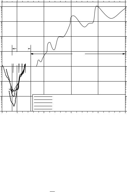
Figure 6.17 Absorption coe cient for pure water as a function of wavelength λ of the radiation. Redrawn from Morel (1974: 18, 19). See Morel (1974) for references.
in water than in air, some light is reflected at the sea surface. For light shining straight down on the sea, the reflectivity is (n − 1)2/(n + 1)2. For seawater, the reflectivity is 0.02 = 2%. Hence most sunlight reaching the sea surface is transmitted into the sea, little is reflected. This means that sunlight incident on the ocean in the tropics is mostly absorbed below the sea surface.
The rate at which sunlight is attenuated determines the depth which is lighted and heated by the sun. Attenuation is due to absorption by pigments and scattering by molecules and particles. Attenuation depends on wavelength. Blue light is absorbed least, red light is absorbed most strongly. Attenuation per unit distance is proportional to the radiance or the irradiance of light:
dI |
= −c I |
(6.13) |
dx |
where x is the distance along beam, c is an attenuation coe cient (figure 6.17), and I is irradiance or radiance.
Radiance is the power per unit area per solid angle. It is useful for describing the energy in a beam of light coming from a particular direction. Sometimes we want to know how much light reaches some depth in the ocean regardless of
6.10. LIGHT IN THE OCEAN AND ABSORPTION OF LIGHT |
99 |
Transmittance (%/m)
100 |
I |
9 |
-0 |
|
|
|
5 |
|
|
||
|
|
|
|
||
80 |
II |
1 |
|
|
|
|
-40 |
|
|||
|
1 |
III |
|
||
|
|
|
|
||
60 |
III |
II |
|
Depth |
|
3 |
-80 |
||||
|
|||||
|
|
|
|
||
|
|
IB |
|
(m) |
|
40 |
5 |
|
|
||
|
|
|
|||
|
IA |
|
|
||
|
|
|
|
||
20 |
7 |
I |
-120 |
|
|
|
|
|
|||
|
9 |
|
|
|
|
0 |
|
|
-160 |
|
300 |
400 |
500 |
600 |
700 |
0.5 1 |
2 |
5 |
10 |
20 |
50 |
100 |
|
|
Wavelength (nm) |
|
|
|
|
Percentage |
|
|
|
|
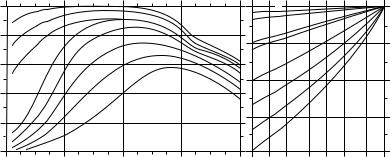
Figure 6.18 Left: Transmittance of daylight in the ocean in % per meter as a function of wavelength. I: extremely pure ocean water; II: turbid tropical-subtropical water; III: mid-latitude water; 1-9: coastal waters of increasing turbidity. Incidence angle is 90◦for the first three cases, 45◦for the other cases. Right: Percentage of 465 nm light reaching indicated depths for the same types of water. After Jerlov (1976).
which direction it is going. In this case we use irradiance, which is the power per unit area of surface.
If the absorption coe cient is constant, the light intensity decreases exponentially with distance.
I2 = I1 exp(−cx) |
(6.14) |
where I1 is the original radiance or irradiance of light, and I2 is the radiance or irradiance of light after absorption.
Clarity of Ocean Water Sea water in the middle of the ocean is very clear— clearer than distilled water. These waters are a very deep, cobalt, blue—almost black. Thus the strong current which flows northward o shore of Japan carrying very clear water from the central Pacific into higher latitudes is known as the Black Current, or Kuroshio in Japanese. The clearest ocean water is called Type I waters by Jerlov (figure 6.18). The water is so clear that 10% of the light transmitted below the sea surface reaches a depth of 90 m.
In the subtropics and mid-latitudes closer to the coast, sea water contains more phytoplankton than the very clear central-ocean waters. Chlorophyll pigments in phytoplankton absorb light, and the plants themselves scatter light. Together, the processes change the color of the ocean as seen by observer looking downward into the sea. Very productive waters, those with high concentrations of phytoplankton, appear blue-green or green (figure 6.19). On clear days the color can be observed from space. This allows ocean-color scanners, such as those on SeaWiFS, to map the distribution of phytoplankton over large areas.
As the concentration of phytoplankton increases, the depth where sunlight is absorbed in the ocean decreases. The more turbid tropical and mid-latitude waters are classified as type II and III waters by Jerlov (figure 6.18). Thus the depth where sunlight warms the water depends on the productivity of the waters. This complicates the calculation of solar heating of the mixed layer.
Coastal waters are much less clear than waters o shore. These are the type 1–9 waters shown in figure 6.18. They contain pigments from land, sometimes
100 |
CHAPTER 6. TEMPERATURE, SALINITY, AND DENSITY |
Reflectance (%)
4
3 |
|
0.3 |
( < 0.1) |
1.3 |
|
2 |
|
0.6
 3.0
3.0
1
0
0.400 |
0.500 |
0.600 |
0.700 |
Wavelength ( m)
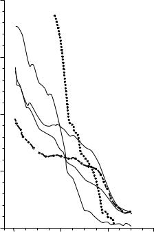
Figure 6.19 Spectral reflectance of sea water observed from an aircraft flying at 305 m over waters of di erent colors in the Northwest Atlantic. The numerical values are the average chlorophyll concentration in the euphotic (sunlit) zone in units of mg/m3. The reflectance is for vertically polarized light observed at Brewster’s angle of 53◦. This angle minimizes reflected skylight and emphasizes the light from below the sea surface. After Clarke, Ewing, and Lorenzen (1970).
called gelbsto e, which just means yellow stu , muddy water from rivers, and mud stirred up by waves in shallow water. Very little light penetrates more than a few meters into these waters.
Measurement of Chlorophyll from Space The color of the ocean, and hence the chlorophyll concentration in the upper layers of the ocean has been measured by the Coastal Zone Color Scanner carried on the Nimbus-7 satellite launched in 1978, by the Sea-viewing Wide Field-of-view Sensor (SeaWiFS) carried on SeaStar, launched in 1997, and on the Moderate Resolution Imaging Spectrometer (modis) carried on the Terra and Aqua satellites launched in 1999 and 2002 respectively. modis measures upwelling radiance in 36 wavelength bands between 405 nm and 14,385 nm.
Most of the upwelling radiance seen by the satellite comes from the atmosphere. Only about 10% comes from the sea surface. Both air molecules and aerosols scatter light, and very accurate techniques have been developed to remove the influence of the atmosphere.