

§6. A Qualitative Method for First Order Equations
The qualitative method developed earlier for autonomous equations is extended to first order equations.
For non-autonomous equations the derivative depends directly on the independent variable as well as the solution. The direction field can still be plotted, but the possible behavior of the solutions can be more complicated than before.
Example 6–1. Suppose a population with unlimited food supply is also subject to (net) emigration. If the emigration is at a variable rate one possible model could be
dtd P(t) = 0.1P(t) − t.
The objective is to study the solutions of this equation without actually finding the formula for the solution.
Exercise 6–1. What is the exact solution of this equation?
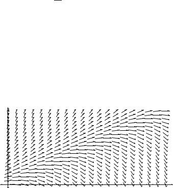
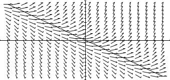
The direction field for this equation is as follows.
Direction Field Plot
500 |
|
|
|
|
|
|
400 |
|
|
|
|
|
|
300 |
|
|
|
|
|
|
P |
|
|
|
|
|
|
200 |
|
|
|
|
|
|
100 |
|
|
|
|
|
|
0 |
10 |
20 |
t |
30 |
40 |
50 |
As before, the qualitative behavior of the solution with given initial value can be sketched from the direction field by following the arrows.
Exercise 6–2. Sketch the solution satisfying the initial condition P(0) = 200.
A more careful examination of the direction field shows that the long run behavior of the solution depends on the intial population size. For example, the
Copyright 2002 Jerry Alan Veeh. All rights reserved.
§6: A Qualitative Method for First Order Equations 38
solution with P(0) = 50 is graphed as follows.
Solution with P(0)=50
500 |
|
|
|
|
|
|
400 |
|
|
|
|
|
|
300 |
|
|
|
|
|
|
P |
|
|
|
|
|
|
200 |
|
|
|
|
|
|
100 |
|
|
|
|
|
|
0 |
10 |
20 |
t |
30 |
40 |
50 |
The graph clearly shows that the population becomes extinct in this case.
In the case of autonomous equations, a central role was played by constant function solutions. These equilibrium solutions were used to determine the limiting behavior of a solution of the equation from its intial value. As is the case for the present equation, non-autonomous equations usually do not have constant function solutions. For these equations the role of the equilibrium solution is played graphically by the zero-cline, which is the curve along which the slope of the solution is zero. It is important to keep in mind that the zero-cline is usually not a solution of the equation.
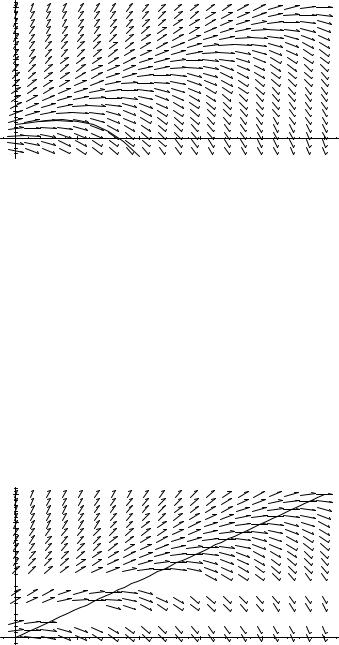
For the equation P′(t) = 0.1P(t) − t the zero-cline is the curve P(t) = 10t. The graph of the direction field and the zero-cline is as follows.
Direction Field Plot with Zero-Cline
500
400
300
P
200
100
0 |
10 |
20 t 30 |
40 |
50 |
The zero-cline always divides the direction field plot into two regions. In one region the direction field has positive slope; in the other region the direction field has negative slope. In this particular case the region of positive slope is above the zero-cline while the region of negative slope is below the zero-cline. Simple reasoning from the differential equation shows that any solution which starts at
§6: A Qualitative Method for First Order Equations 39
t = 0 with a slope exceeding 10 will never cross the zero-cline. Such a solution will tend to infinity. A solution starting at time t = 0 with a slope of less than 10 will eventually cross the zero-cline. Once this occurs, the solution will diverge to minus infinity. This analysis shows that the initial population size must be at least 100 if the population is to avoid extinction.
Exercise 6–3. Verify the conclusion of the graphical analysis by examining the behavior of the exact solution obtained earlier.
It is not always possible to perform such a detailed graphical analysis in the general case. Usually at least some aspects of the behavior of the solutions can be obtained using these simple graphical methods.
§6: A Qualitative Method for First Order Equations 40
Problems
Problem 6–1. What characteristic of a direction field will identify it as the direction field of an autonomous equation?
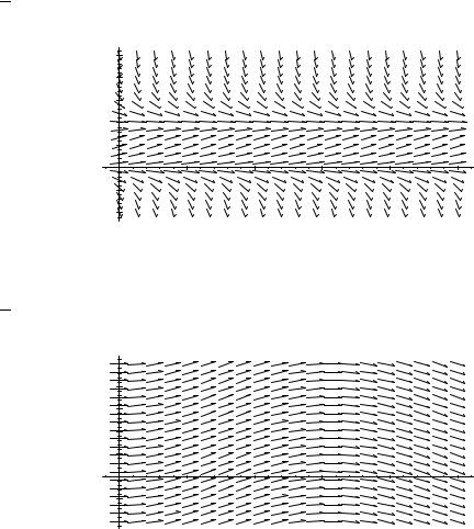
Problem 6–2. The function A(t) satisfies a first order differential equation which has direction field A below. Sketch the solution satisfying the initial condition A(0) = 5 for 0 ≤ t ≤ 4.
Problem 6–3. The function B(t) satisfies a first order differential equation which has direction field B below. Sketch the solution satisfying the initial condition B(0) = 3 for 0 ≤ t ≤ 4.
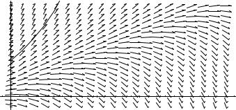
Problem 6–4. Could direction field A below come from the differential equation dtd A(t) = A(t)(2 − A(t))? Why?
Direction Field Plot A
5 |
|
|
|
|
|
|
4 |
|
|
|
|
|
|
A 3 |
|
|
|
|
|
|
2 |
|
|
|
|
|
|
1 |
|
|
|
|
|
|
0 |
1 |
2 |
t |
3 |
4 |
5 |
-1 |
|
|
|
|
|
|
-2 |
|
|
|
|
|
|
Problem 6–5. Could direction field B below come from the differential equation dtd B(t) = sin B(t)? Why?
Direction Field Plot B
5 |
|
|
|
|
|
|
4 |
|
|
|
|
|
|
B 3 |
|
|
|
|
|
|
2 |
|
|
|
|
|
|
1 |
|
|
|
|
|
|
0 |
1 |
2 |
t |
3 |
4 |
5 |
-1 |
|
|
|
|
|
|
-2 |
|
|
|
|
|
|
Problem 6–6. Consider the equation x′(t) − x(t) = t. Make a rough sketch of the direction field, showing the isocline corresponding to zero slope and indicating
§6: A Qualitative Method for First Order Equations 41
where the direction field has positive and negative slope. If x(0) = 3, what is |
|
lim x(t)? If x(0) = −3, what is lim x(t)? |
|
t→∞ |
t→∞ |
§6: A Qualitative Method for First Order Equations 42
Solutions to Problems
Problem 6–1. Since for an autonomous equation the derivative of the function does not depend on the independent variable, the direction field will not depend on the independent variable either.
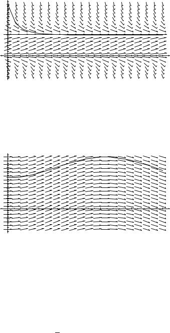
Problem 6–2.
Solution with A(0)=5
5 |
|
|
|
|
|
|
4 |
|
|
|
|
|
|
A 3 |
|
|
|
|
|
|
2 |
|
|
|
|
|
|
1 |
|
|
|
|
|
|
0 |
1 |
2 |
t |
3 |
4 |
5 |
-1 |
|
|
|
|
|
|
-2 |
|
|
|
|
|
|
Problem 6–3.
Solution with B(0)=3
5 |
|
|
|
|
|
|
4 |
|
|
|
|
|
|
B 3 |
|
|
|
|
|
|
2 |
|
|
|
|
|
|
1 |
|
|
|
|
|
|
0 |
1 |
2 |
t |
3 |
4 |
5 |
-1 |
|
|
|
|
|
|
-2 |
|
|
|
|
|
|
Problem 6–4. Direction field A has 2 equilibrium solutions, one at 0 and the other at 2. The equilibrium solution at 2 is stable while the solution at 0 is unstable. The sign of the derivative as given in plot A as well as the equilibrium solutions agree with those of the given equation. The answer is yes.
Problem 6–5. Direction field plot B does not depend on the value of B(t) since the field lines are all parallel. The answer is no. It is more likely that plot B corresponds to the equation dtd B(t) = sin t.
§6: A Qualitative Method for First Order Equations 43
Problem 6–6.
4
2
-4 -2 0 2t 4
2t 4
-2 -4
From the direction field, if x(0) = 3 then limt→∞ x(t) = ∞. From the direction
field lim x(t) = −∞ in the case x(0) = −3.
t→∞
§6: A Qualitative Method for First Order Equations 44
Solutions to Exercises
Exercise 6–1. Using the integrating factor e−t/10 after rewriting the equation shows that the general solution is P(t) = 10t + 100 + Cet/10.
Exercise 6–2. Simply follow the arrows, keeping in mind that the arrows are tangent to the solution curve at each point. The graph should be as follows.
Solution with P(0)=200
500 |
|
|
|
|
|
|
400 |
|
|
|
|
|
|
300 |
|
|
|
|
|
|
P |
|
|
|
|
|
|
200 |
|
|
|
|
|
|
100 |
|
|
|
|
|
|
0 |
10 |
20 |
t |
30 |
40 |
50 |
Exercise 6–3. Writing the solution found earlier by evaluating the unknown constant in terms of the initial population size gives P(t) = 10t + 100 + (P(0) − 100)et/10. Hence if P(0) > 100, the population size increases indefinitly, while if P(0) < 100, extinction occurs.