

§10. Systems of First Order Equations
Systems of first order differential equations arise in many contexts. The qualitative methods developed earlier can be used to understand some of the basic properties of the solutions of a system.
The first example illustrates a situation which gives rise to a system (pair) of differential equations.
Example 10–1. The classical Lotka-Volterra predator-prey model can be described as follows. An ecosystem contains 2 different species A and B. Species A is a predator that feeds on species B and only on species B. Species B depends only on the enviroment for nutrition and nutrition is unlimited. Denote by A(t) and B(t) the population sizes for the 2 species at time t. A possible model is then provided by the system of differential equations
d
dt d
dt
The constants kA and kB represent the growth rates of the individual species populations in the absence of the other species. Thus kA < 0 and kB > 0 here. The constants e and f reflect the interdependency of the 2 species. The product A(t)B(t) measures the chances of interaction between members of the two species. In the present context, the constant e should be positive while f should be negative.
Exercise 10–1. Why is e > 0 reasonable? Why is f < 0 reasonable? Why should kA < 0 and kB > 0 hold?
The system can be expressed in vector form as
d
dt (A(t), B(t)) = (kAA(t) + eA(t)B(t), f A(t)B(t) + kBB(t)) which is reminicent of equations studied earlier.
The Lotka-Volterra system is an example of an autonomous system since the independent variable t appears only through the unknown functions A(t) and B(t).
Qualitative information about the solution of the system can be obtained by methods similar to those used earlier.
Example 10–2. Suppose a Lotka-Volterra model for the predator-prey population is given by
dtd (A(t), B(t)) = (−0.10A(t) + 0.01A(t)B(t), −0.01A(t)B(t) + 0.03B(t))
Copyright 2002 Jerry Alan Veeh. All rights reserved.
§10: Systems of First Order Equations 62
with the initial population A(0) = 5 and B(0) = 30. What is the population dynamics?
In parallel with the analysis in the one dimensional case, the first step in the analysis is to find the equilibrium solutions. This is done by setting the derivative vector equal to the zero vector and solving for A(t) and B(t). In this case, the two equilibrium solutions are A(t) = B(t) = 0 for all t, and A(t) = 3 and B(t) = 10 for all t.
Exercise 10–2. Verify that these are the only two equilibrium solutions.
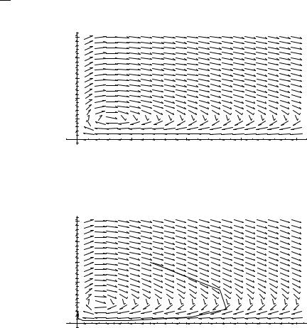
The second step is to plot the direction field. Since the system is autonomous, the derivative vector depends only on the values of the unknown functions. The direction field is then obtained by plotting a vector of length one proportional to
dtd (A(t), B(t)) at each point in the A-B plane.
Direction Field for Lotka-Volterra Model
50 |
|
|
|
|
40 |
|
|
|
|
30 |
|
|
|
|
B |
|
|
|
|
20 |
|
|
|
|
10 |
|
|
|
|
0 |
5 |
10 |
15 |
20 |
|
|
A |
|
|
As before, once the direction field is drawn, the behavior of a solution starting from any given initial conditions can be sketched by following the arrows.
Solution with A(0)=10 B(0)=30
50 |
|
|
|
|
|
|
40 |
|
|
|
|
|
|
30 |
|
|
|
|
|
|
B |
|
|
|
|
|
|
20 |
|
|
|
|
|
|
10 |
|
|
|
|
|
|
0 |
5 |
10 |
15 |
20 |
25 |
30 |
|
|
|
A |
|
|
|
Example 10–3. The Maple command to draw the direction field for the last example is
DEplot({diff(A(t), t) = −0.1 A(t) + 0.01 A(t) B(t),
diff(B(t), t) = −.01 A(t) B(t) + 0.03 B(t)}, [A(t), B(t)], 0..100, A = 0..30, B = 0..50);
§10: Systems of First Order Equations 63
and a solution starting with specified initial conditions is obtained with
DEplot({diff(A(t), t) = −0.1 A(t) + 0.01 A(t) B(t), diff(B(t), t) = −x.01 A(t) B(t) + 0.03 B(t)},
[A(t), B(t)], 0..100, [[A(0) = 10, B(0) = 30]], A = 0..30, B = 0..50);.

§10: Systems of First Order Equations 64
Problems
Problem 10–1. Two countries, A and B, are suspicious of each other and respond by building up armaments. Suppose A(t) and B(t) are the arms budgets of the two countries at time t. Find a simple model that describes the growth of the arms budgets through time.
Problem 10–2. For the system
dtd A(t) = −0.2A(t) + 0.9B(t) + 10 dtd B(t) = 0.9A(t) − 0.2B(t) + 20
find the equilibrium solution. Is the equilibrium solution stable or unstable? Justify your answer.
Problem 10–3. Suppose that each of the two species in the example would follow logistic growth if the other species were absent. What would the system be in this case?
§10: Systems of First Order Equations 65
Solutions to Problems
Problem 10–1. The basic rationale would be as follows. The rate of growth of the arms budget of country A is proportional to the arms budget of country B since the size of B’s budget represents a threat. However, arms cost money, so this rate is also proportional to A’s arms budget. There is also a constant growth factor representing inflation. A similar reasoning applies to country B. A simple model with these characteristics could be
dtd A(t) = −aA(t) + bB(t) + c dtd B(t) = dA(t) − f B(t) + g
where all of the constants are positive.
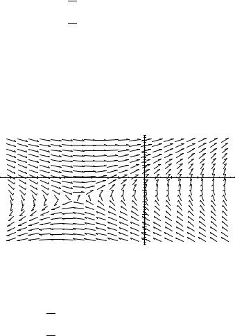
Problem 10–2. The equilibrium solution occurs when A = −25.97 and B = −16.88. This solution is unstable, as is seen from the direction field plot: a small disturbance away from the equilibrium will cause the solution to move off to infinity or minus infinity.
|
|
|
Problem 10-2 |
|
|
|
|
|
|
|
|
|
30 |
|
|
|
|
|
|
|
20 |
|
|
-50 |
-40 |
-30A |
-20 |
-10 |
10 |
20 |
30 |
10 |
|||||||
|
|
|
|
|
0 |
|
|
|
|
|
|
|
-10 |
|
|
|
|
|
|
|
-20 |
|
|
|
|
|
|
|
B |
|
|
|
|
|
|
|
-30 |
|
|
|
|
|
|
|
-40 |
|
|
|
|
|
|
|
-50 |
|
|
Problem 10–3.
d
dt A(t) = kAA(t)(MA − A(t)) + eA(t)B(t)
d
dt B(t) = f A(t)B(t)(MB − B(t)) + kBB(t).
§10: Systems of First Order Equations 66
Solutions to Exercises
Exercise 10–1. Since species A is the predator, the more interactions between predator and prey, the better for species A. This explains why e > 0. These interactions are bad for species B, so f < 0. On the other hand, the more predators there are, the harder it will be for each one to find sufficient food. Thus kA < 0. The more prey there are, the easier it will be for each one to avoid capture. Hence kB > 0.
Exercise 10–2. Just plug the proposed solutions into the system of equations.