§5. The General First Order Linear Equation

The integrating factor method of solving the general first order linear equation is discussed.

Example 5–1. A rocket is launched at time t = 0 and its engine provides a constant thrust for 10 seconds. During this time the burning of the rocket fuel constantly decreases the mass of the rocket. The problem is to determine the velocity v(t) of the rocket at time t during this initial 10 second interval. Denote by m(t) the mass of the rocket at time t and by U the constant upward thrust (force) provided by the engine. Applying Newton’s Law gives

dtd (m(t)v(t)) = U − kv(t) − m(t)g

where an air resistance term is included in addition to the gravitational and thrust terms. This equation is linear, non-homogeneous, and not autonomous. How is this equation solved?

The method is called the integrating factor technique.

(1) Re-arrange the equation as necessary to be in the form dtd v(t)+a(t)v(t) = b(t). The coefficient of the derivative term must be 1.

(2)Compute the integrating factor e a(t) dt. The integral here can use any antiderivative of a(t).

(3)Multiply both sides of the equation obtained in step 1 by the integrating factor. The result is guaranteed to be in the form

(4)Integrate both sides and solve for the unknown function. Use the initial condition and the Fundamental Theorem of Calculus.

To illustrate the method of solution the simpler equation

dtd v(t) = tv(t) + t

or

dtd v(t) − tv(t) = t

with initial condition v(0) = 0 is studied first. The integrating factor here is e −t dt. Multiply both sides of the equation by this factor. After multiplication the left side

Copyright 2002 Jerry Alan Veeh. All rights reserved.

§5: The General First Order Linear Equation 31

of the equation will be the derivative of a product of the integrating factor and the unknown function v(t). This gives the equation

dtd e−t2/2v(t) = te−t2/2.

Both sides can now be integrated with respect to t from 0 to s. Using the Fundamental Theorem of Calculus on the left hand side, this gives

e−s2/2v(s) − e02/2v(0) = s e−t2/2 dt.

0

The integral on the right side can be integrated by substitution to give 1 − e−s2/2. Using this fact and the initial condition v(0) = 0, the equation above can now be

solved to give

v(s) = es2/2(1 − e−s2/2) = es2/2 − 1.

Exercise 5–1. Verify carefully all of the steps in this derivation.

The integrating factor technique will solve any first order linear equation, and thus provides yet another method of solving first order linear equations with constant coefficients and also certain autonomous equations. The success of the method depends on the ability to compute the two integrals that arise. Since the second integral is a definite integral, numerical methods can be used to find the value of the solution at any particular point.

Example 5–2. The equation dtd v(t) = tv(t) + t2 with initial condition v(0) = 5 will be solved. First, the equation is rewritten as dtd v(t) − tv(t) = t2 and the integrating factor

e−t2/2 is found. Multiplying by the integrating factor gives dtd e−t2 /2v(t) = t2e−t2/2. Now integrate both sides from 0 to s to obtain

s

e−s2/2v(s) − 5e−02/2 = t2e−t2/2 dt

0

or

s

v(s) = 5 + es2/2 t2e−t2 /2 dt.

0

This last expression can be used together with Simpson’s Rule, or another numerical integration technique, to numerically compute the value of v at any particular s.

Example 5–3. As the final example, the general solution of the general first order linear equation will be found. As above, the equation is first written as v′(t) + a(t)v(t) = b(t) and the initial condition is assumed to be the value v(t0) for some point t0. To make the computations simpler, the integrating factor is taken as

t

the definite integral e t0 a(r) dr. Multiplying by the integrating factor transforms

§5: The General First Order Linear Equation 32

Theorem and the initial condition to integrate both sides of this equation from 0 to

Although this expression is complicated, the connection between the initial condition, the function b(t), and the solution v(s) is clearly displayed.

§5: The General First Order Linear Equation 34

Problem 5–10. Garfield the cat is on a diet. His basic metabolism consumes 200 calories per day. His exercise program consumes 100 calories per day per kilogram of body mass. Food intake provides 750 calories per day. Caloric intake that is not consumed by basic metabolism or exercise is converted into fat; calories needed for basic metabolism or exercise in excess of caloric intake are obtained from the fat store. Body fat stores or releases calories at a rate of 5,000 calories per kilogram of fat. Assume that the conversion of calories to fat (and vice-versa) is perfectly efficient. Denote by G(t) the mass, in kilograms, of Garfield on day t of this diet regimen. Write a differential equation for G(t) using the information given. If Garfield sticks religiously to this diet, what is his ultimate mass?

§5: The General First Order Linear Equation 35

Solutions to Problems

Problem 5–1. Using the general form of the last example with a(t) = −2t and

Problem 5–2. The integrating factor is e−3t so that finally y(t) = (−5/2)e3t − (1/2)et.

Problem 5–3. The constant function solutions are the constant function 0 and the constant function 7. If 0 < C(t) < 7, C′(t) > 0 and so the function C(t)

increases toward the value 7. Hence lim C(t) = 7.

t→∞

Problem 5–4. Rewriting the equation as B′(t) − B(t) = e2t shows that the integrating factor is e−t, so that after multiplying by the integrating factor the equation becomes (e−tB(t))′ = et. Integration from 0 to t gives e−tB(t) − B(0) = et − 1 so that B(t) = e2t after using the initial condition. The limit is infinity.

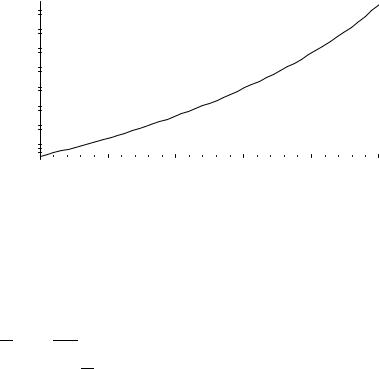
Problem 5–5. The equation to be solved is dtd ((11 − t)v(t)) = 200 − (11 − t)g.

Since the right side does not depend on v(t), the equation can be solved by

simple integration. The final solution as v(t) = 200t + (g/2)(11 − t)2 − 121g/2 11 − t

for 0 ≤ t ≤ 10.

Problem 5-5

1400

1200

1000

800

600

400

200

§5: The General First Order Linear Equation 36

t)g ln(11 − t) − (200/11 + g ln(11))(11 − t).

Problem 5-6

160

140

120

100

80

60

40

20

Problem 5–8. The differential equation for the amount A(t) in the account is dtd A(t) = 5100+ t A(t) + 1000 + 100t with A(0) = 0. The contributions C(t) up to time t satisfies dtd C(t) = 1000 + 100t with C(0) = 0. The C equation is solved

easily by integration to give C(t) = 1000t + 50t2 and so C(2) = 2200. The integrating factor for the A equation is e−(5+t)2/200. Using definite integrals from

0 to s then gives A(s) = e(5+s)2/200 s(1000 + 100t)e−(5+t)2/200 dt. Plugging in s = 2

0

and integrating numerically gives A(2) = 2, 340.99.

Problem 5–9. Let C(t) be the number of pounds of dissolved chlorine in the pool after t days. Assume that a tablet dissolves at a constant rate. This means that each tablet supplies chlorine at a rate of 1/20 pound per day for 0 ≤ t ≤ 5. Also assume that the dissolved chlorine is instantly mixed throughout the pool. In one day, 500 × 24 = 12, 000 gallons of mixture leaves the pool and is replaced by fresh water. Hence C′(t) = N/20 − (12, 000/50, 000)C(t) where N is the number of quarter pound tablets. Since C(0) = 0, this equation can be solved and the value of N required so that C(3) = 2 can then be found.

Problem 5–10. Computing in terms of calories gives the equation 5000G′(t) = 750 − 200 − 100G(t). The constant function solution of the differential equation is G(t) = 5.5 kilograms, which from the direction field is the ultimate mass for Garfield.