

§4. A Qualitative Method for First Order Autonomous Equations
The intuition behind Euler’s method can also be used to develop a visual technique for studying the behavior of solutions of a differential equation. This method applied to first order autonomous equations is developed here.
Example 4–1. The equation P′(t) = 0.001P(t)(1000 − P(t)) is the logistic equation of population growth. What are the basic properties of the solution? Even though the solution can be explicitly found, the basic properties of the solution can be difficult to determine from the final form of the solution.
Exercise 4–1. Find the general solution of this equation.
Euler’s method was based on the observation that the differential equation gives a formula for the derivative of the unknown function in terms of the values of the unknown function. Instead of using the Fundamental Theorem of Calculus to develop a computational formula, recall instead that one interpretation of the derivative of a function is as the slope of graph of function at a point. Hence the differential equation gives a formula for the slope of the graph of the function in terms of the value of the function. This observation suggests the following graphical method. At each point (t, P(t)), use the differential equation to compute the slope P′(t) of the solution which passes through this point. Represent this slope on the two dimensional grid by drawing an arrow at the point (t, P(t)) having slope P′(t). The graph consisting of all of these arrows then gives the slope of the solution at any particular point. This arrow plot is called the direction field plot of the differential equation. The solution can then be graphed by following the arrows.
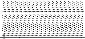
A computer can be easily programmed to do the calculations and plotting. The direction field for the equation P′(t) = 0.001P(t)(1000 − P(t)) is as follows.
Direction Field Plot
1400 |
|
|
|
|
|
|
1200 |
|
|
|
|
|
|
1000 |
|
|
|
|
|
|
800 |
|
|
|
|
|
|
P |
|
|
|
|
|
|
600 |
|
|
|
|
|
|
400 |
|
|
|
|
|
|
200 |
|
|
|
|
|
|
0 |
1 |
2 |
t |
3 |
4 |
5 |
To illustrate one specific computation for this equation, consider |
the point (0, 1) |
in the graph of the function P(t). This point corresponds to the |
solution taking |
Copyright 2002 Jerry Alan Veeh. All rights reserved.

§4: A Qualitative Method for First Order Autonomous Equations 23
the value P(0) = 1 at t = 0. The slope of the solution through this point is P′(0) = 0.001(1)(1000 − 1) = 0.999. So the arrow at the point (0, 1) should have slope 0.999.
Exercise 4–2. What is the slope of the arrow at the point (3, 10)?
With the direction field in hand, any single solution can be graphed easily. For example, the solution satisfying P(0) = 100 is sketched by beginning at the point (0, 100) and following the arrows.
Solution with P(0)=100
1400 |
|
|
|
|
|
|
1200 |
|
|
|
|
|
|
1000 |
|
|
|
|
|
|
800 |
|
|
|
|
|
|
P |
|
|
|
|
|
|
600 |
|
|
|
|
|
|
400 |
|
|
|
|
|
|
200 |
|
|
|
|
|
|
0 |
1 |
2 |
t |
3 |
4 |
5 |
Exercise 4–3. What is the graph of the solution satisfying P(0) = 500?
Exercise 4–4. What is the graph of the solution satisfying P(0) = 2000? What is
lim P(t) in this case?
t→∞
As is seen in the preceding exercises, the direction field plot allows all solutions to be studied simultaneously. Features that are common to all solutions can then be identified. These common features often center around the constant function solutions. A reasonable first step in studying a differential equation is to find all solutions which are constant functions. These solutions are called the equilibrium solutions. For the equation of the previous example, equilibrium solutions are found
by replacing dtd P(t) with 0 and then solving for P(t). In the previous example, the constant functions which solve the equation are the zero solution and the function which always takes the value 1000.
Exercise 4–5. Verify that if P(t) = 0 for all t > 0 then P(t) solves the equation. Do the same if P(t) = 1000 for all t > 0.
The constant function solution P(t) = 1000 is a stable equilibrium. This is because any solution which takes values near 1000 will approach 1000 in the limit as t → ∞. The constant function solution P(t) = 0 is an unstable equilibrium. Any
§4: A Qualitative Method for First Order Autonomous Equations 24
solution taking values near 0 (but not equal to 0) will tend in the limit as t → ∞ to either 1000 or −∞, not to 0.
Exercise 4–6. Is it always true that the direction field for an autonomous equation is the same along any two vertical lines?
Example 4–2. The Maple command to plot the direction field for the equation x′(t) = x(t) is
DEplot({diff(x(t), t) = x(t)}, {x(t)}, t = −3..3, x = −10..10);.
§4: A Qualitative Method for First Order Autonomous Equations 25
Problems
Problem 4–1. For the population model dtd P(t) = 5P(t)(1000 − P(t)) with P(0) =
100 find the asymptotic population size lim P(t).
t→∞
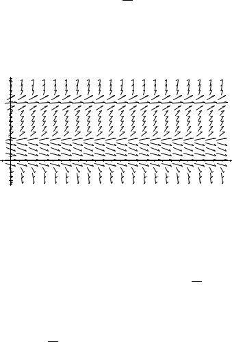
Problem 4–2. Suppose a first order autonomous equation has direction field
Direction Field Plot
40 |
|
|
|
|
|
|
30 |
|
|
|
|
|
|
A20 |
|
|
|
|
|
|
10 |
|
|
|
|
|
|
0 |
1 |
2 |
t |
3 |
4 |
5 |
-10 |
|
|
|
|
|
|
What are the equilibrium solutions? Which of the equilibrium solutions are stable? What is the asymptotic behavior of a solution satisfying A(0) = 1? Satisfying A(0) = 15? Give one equation for which this plot could be the direction field.
Problem 4–3. Suppose a > 0 and b > 0 are constants and dtd P(t) = aP(t)− b(P(t))2 for t > 0. Describe the behavior of a solution which has a positive value at time t = 0. Your answer will depend on a and b.
Problem 4–4. Suppose dtd x(t) = (1 − x(t))(2 − x(t))(3 − x(t)) for t > 0. Sketch the direction field for this equation. What is the asymptotic behavior of the solution which satisfies x(0) = 3/ 2? What if x(0) = 4? If x(0) = −5?
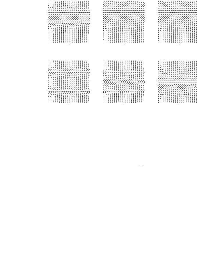
Problem 4–5. For each of the equations below, give the letter corresponding to its direction field plot. Also compute the indicated limit if x(0) = 0.
(a) For the equation x′(t) |
= |
x(t) − 2 the direction field plot is |
|
|
|
|
|
and |
|
|
|
||||||
lim x(t) = |
|
|
|
|
|
|
|
|
t→∞ |
|
|
|
|
|
|
|
|
(b) For the equation x′(t) |
= |
x(t)2 − 4 the direction field plot is |
|
|
|
and |
||
|
|
|
||||||
lim x(t) = |
|
|
|
|
|
|
|
|
t→∞ |
|
|
|
|
|
|
|
|
(c) For the equation x′(t) = x(t)3 − 4x(t) the direction field plot is |
|
|
|
and |
||||
|
|
|
||||||
lim x(t) = |
|
|
|
|
|
|
|
|
t→∞ |
|
|
|
|
|
|
|
|
§4: A Qualitative Method for First Order Autonomous Equations 26
|
|
Plot A |
|
|
|
|
4 |
|
|
|
|
x(t)2 |
|
|
-4 |
-2 |
0 |
2t |
4 |
|
|
-2 |
|
|
|
|
-4 |
|
|
|
|
Plot D |
|
|
|
|
4 |
|
|
|
|
x(t)2 |
|
|
-4 |
-2 |
0 |
2t |
4 |
|
|
-2 |
|
|
|
|
-4 |
|
|
|
|
Plot B |
|
|
|
|
4 |
|
|
|
|
x(t)2 |
|
|
-4 |
-2 |
0 |
2t |
4 |
|
|
-2 |
|
|
|
|
-4 |
|
|
|
|
Plot E |
|
|
|
|
4 |
|
|
|
|
x(t)2 |
|
|
-4 |
-2 |
0 |
2t |
4 |
|
|
-2 |
|
|
|
|
-4 |
|
|
|
|
Plot C |
|
|
|
4 |
|
|
|
x(t)2 |
|
-4 |
-2 |
0 |
2t |
|
|
-2 |
|
|
|
-4 |
|
|
|
Plot F |
|
|
|
4 |
|
|
|
x(t)2 |
|
-4 |
-2 |
0 |
2t |
|
|
-2 |
|
|
|
-4 |
|
Problem 4–6. Solve the equation A′(t) = 1+A(t) with the initial condition A(0) = 0.
What is lim A(t)?
t→∞
Problem 4–7. Can the function x(t) = sin t be a solution of the equation |
d |
x(t) = |
|
dt |
|||
1 − (x(t))2? Why or why not? Hint: What is the direction field? |
|
||
|
|
Problem 4–8. The velocity of a falling body of mass m in the presence of air resistance was earlier found to satisfy the equation mdtd v(t) = −kv(t) − mg. Plot the direction field for v(t). What are the equilibrium solutions, and which are stable? What is the asymptotic velocity of the falling body?
§4: A Qualitative Method for First Order Autonomous Equations 27
Solutions to Problems
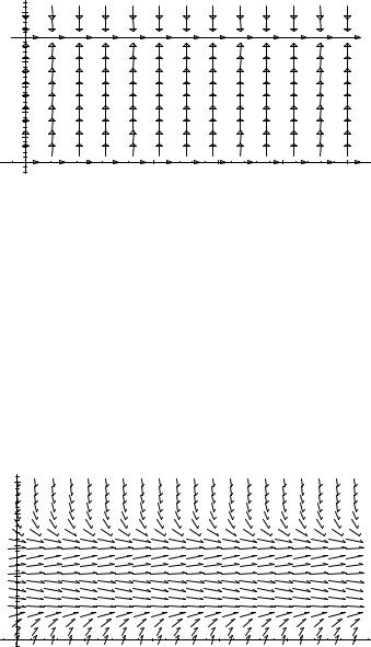
Problem 4–1. The equilibrium solutions are again 0 and 1000. The direction field is
Direction Field Plot
1200 |
|
|
|
|
|
|
1000 |
|
|
|
|
|
|
800 |
|
|
|
|
|
|
P |
|
|
|
|
|
|
600 |
|
|
|
|
|
|
400 |
|
|
|
|
|
|
200 |
|
|
|
|
|
|
0 |
1 |
2 |
t |
3 |
4 |
5 |
Thus the asymptotic population size is 1000.
Problem 4–2. The equilibrium solutions are 0, 10, and 100 and none are stable. A solution with A(0) = 1 will have asymptotic value 0; a solution with A(0) = 15 will have asymptotic value 100. One such equation is A′(t) = A(t)2(A(t) − 10)(A(t) − 30)2.
Problem 4–3. In this case the equilibrium solutions are 0 and a/b, and a/b is a stable equilibrium. The asymptotic value of a solution which has a postive value at t = 0 is therefore a/b.
Problem 4–4. The direction field is
Direction Field Plot
5 |
|
|
|
|
|
|
4 |
|
|
|
|
|
|
x 3 |
|
|
|
|
|
|
2 |
|
|
|
|
|
|
1 |
|
|
|
|
|
|
0 |
1 |
2 |
t |
3 |
4 |
5 |
From the diagram 1 and 3 are stable equilibria, while 2 is unstable. If x(0) = 3/2 the asymptotic value is 1; if x(0) = 4 the asymptotic value is 3; if x(0) = −5 the asymptotic value is 1.
Problem 4–5. In (a) the direction field plot is B and the limit is −∞; in (b) the direction field plot is D and the limit is −2; in (c) the direction field plot is E and the limit is 0.

§4: A Qualitative Method for First Order Autonomous Equations 28
Problem 4–6. Separation of variables gives 1 + A(t) = 1 from which integra-
tion gives ln |1 + A(t)| = t + C. The condition A(0) = 0 gives C = 0 and also allows the removal of the absolute value signs to give A(t) = et − 1. From the
solution or from the direction field, lim A(t) = ∞.
t→∞
Problem 4–7. The direction field shows that 1 is a stable equilibrium while −1 is not. Hence the proposed solution sin t would have to have asymptotic value 1, which precludes oscillation.
Problem 4–8. The equilibrium solution is −mg/k, which is stable. The asymptotic velocity is therefore −mg/k.
§4: A Qualitative Method for First Order Autonomous Equations 29
Solutions to Exercises
Exercise 4–1. By separation of variables |P(t)/(1000 − P(t))| = et+C. How are the absolute value signs removed? What are the constant solutions of the equation?
Exercise 4–2. The slope is P′(3) = 0.001P(3)(1000−P(3)) = 0.001(10)(1000− 10) = 9.90.
Exercise 4–3. Start at the point (0, 500) and follow the arrows. What is limt→∞ P(t) in both of these cases?
Exercise 4–4. The limit is still 1000.
Exercise 4–5. Just substitute these constant solutions in and verify that the equation holds.
Exercise 4–6. Yes. Since the equation is autonomous, the formula for the derivative does not depend on the independent variable alone.