

numerical methods - 4.33
// Loop for trapezoidal integration
//
total = 0; // set the initial sum to zero for i=0:steps,
x = x_start + i * x_delta; if i == 0 then
total = total + f(x); elseif i == steps then
total = total + f(x);
else
total = total + 2 * f(x);
end
end
total = total * x_delta / 2;
printf("Trapezoidal integration value %f\n", total);
//
// Loop for Simpson's rule integration
//
total = 0; // set the initial sum to zero even = 0;
for i=0:steps,
x = x_start + i * x_delta; if i == 0 then
total = total + f(x); elseif i == steps then
total = total + f(x);
else
even = even + 1; if even > 1 then
total = total + 4 * f(x); even = 0;
else
total = total + 2 * f(x);
end
end
end
total = total * x_delta / 3;
printf("Simpsons rule integration value %f\n", total);
Figure 4.32 Integration with a Scilab Program (cont’d)
4.6ADVANCED TOPICS
4.6.1Switching Functions
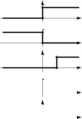
When analyzing a system, we may need to choose an input that is more complex than inputs such as steps, ramps, sinusoids and parabolae. The easiest way to do this is to use switching functions. Switching functions turn on (have a value of 1) when their argu-
numerical methods - 4.34
ments are greater than or equal to zero, or off (a value of 0) when the argument is negative. Examples of the use of switching functions are shown in Figure 4.33. By changing the values of the arguments we can change when a function turns on or off.
u( t)
1
t
 u( –t)
1
t
u( t – 1)
1
t
1  u( t + 1)
|
1 |
|
t |
|
||
|
|
|
|
|
|
|
|
-1 |
|
u( t + 1) – u( t – 1) |
|||
|
|
|
||||
|
|
|
||||
|
|
1 |
|
t |
||
|
|
|
|
|
|
|
|
-1 |
|
|
1 |
|
|
|
|
|
||||
Figure 4.33 Switching function examples
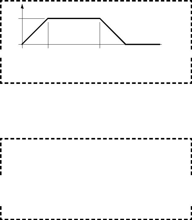
These switching functions can be multiplied with other functions to create a complex function by turning parts of the function on or off. An example of a curve created with switching functions is shown in Figure 4.34.
numerical methods - 4.35
f(t)
5
t  seconds
|
0 |
1 |
3 |
4 |
|
|
|
||||
|
|
|
|
|
|
f( t) = 5t( u( t) – ( t – 1) ) + 5( u( t – 1) – u( t – 3) ) + ( 20 – 5t) ( u( t – 3) – u( t – 4) )
or
f( t) = 5tu( t) – 5( t – 1) u( t – 1) – 5( t – 3) u( t – 3) + 5( t – 4) u( t – 4)
Figure 4.34 Switching functions to create a non-smooth function
The unit step switching function is available in Mathcad and makes creation of complex functions relatively trivial. Step functions are also easy to implement when writing computer programs, as shown in Figure 4.35.
For the function f( t) = 5tu( t) – 5( t – 1) u( t – 1) – 5( t – 3) u( t – 3) + 5( t – 4) u( t – 4)
double u(double t){
if(t >= 0) return 1.0; return 0.0;
}
double function(double t){
|
double |
|
|
|
f; |
|
|
|
|
|
|
f = |
5.0 * t * u(t) |
|
|
|
|
|
|||
|
|
|
|
|
|
|||||
|
|
|
|
|
|
|||||
|
|
- 5.0 |
* (t - 1.0) * u(t - 1.0) |
|
||||||
|
|
- |
5.0 |
* |
(t - 3.0) |
* |
u(t |
- |
3.0) |
|
|
|
|
||||||||
|
|
+ |
5.0 |
* |
(t - 4.0) |
* |
u(t |
- |
4.0); |
|
|
|
|
||||||||
|
|
|
|
|
|
|
|
|
|
|
return f;
}
Figure 4.35 A subroutine implementing the example in Figure 4.34
numerical methods - 4.36
4.6.2 Interpolating Tabular Data
In some cases we are given tables of numbers instead of equations for a system component. These can still be used to do numerical integration by calculating coefficient values as required, in place of an equation.
Tabular data consists of separate data points as seen in Figure 4.36. But, we may need values between the datapoints. A simple method for finding intermediate values is to interpolate with the "lever law". (Note: it is called this because of its’ similarity to the equation for a lever.) The table in the example only gives flow rates for a valve at 10 degree intervals, but we want flow rates at 46 and 23 degrees. A simple application of the lever law gives approximate values for the flow rates.
|
|
|
|
|
|
|
|
|
|
|
|
|
|
|
|
|
|
|
|
|
|
|
|
|
|
|
|
|
|
|
|
|
|
|
|
|
|
|
|
|
|
|
|
|
|
|
|
|
|
|
|
|
|
|
|
|
|
|
|
|
|
|
|
|
|
|
|
|
|
|
valve angle |
|
flow rate |
|
|
|
|
|
|
|
|
|
|
|
|
|
|
|
|
|
|
|
|
|
|
|
|
|
|
|
|
|
|
|
|
|
|
|
|
|
|
|
|
|
|
|
|||||||||||||||||
|
|
|
|
|
|
|
|
|
|
|
|
|
|
|
|
|
|
|
|
|
|
|
|
|
|
|
|
|
|
|
|
|
|
|
|
|
|
|
|
|
|
|
|
|
|
|
|
|||||||||||||||||||
|
|
|
|
|
|
|
|
|
|
|
|
|
|
|
|
|
|
|
|
|
|
|
|
|
|
|
|
|
|
|
|
|
|
|
|
|
|
|
|
|
|
|
|
|
|
|
|
|||||||||||||||||||
|
|
|
|
(deg.) |
|
(gpm) |
|
|
|
|
Given a valve angle of 46 degrees the flow rate is, |
|
|
|
|
|||||||||||||||||||||||||||||||||||||||||||||||||||
|
|
|
|
|
|
|
|
|
|
|
|
|
||||||||||||||||||||||||||||||||||||||||||||||||||||||
|
|
|
|
|
|
|
|
|
|
|
|
|
|
|
|
|
|
|
|
|
|
|
|
|
|
|
|
|
|
|
|
|||||||||||||||||||||||||||||||||||
|
|
|
|
|
|
|
|
|
|
|
|
|
|
|
|
|
|
|
|
|
|
|
|
|
|
|
|
|
|
|
|
|||||||||||||||||||||||||||||||||||
|
|
|
|
0 |
|
|
|
|
|
|
|
|
0 |
|
|
|
|
|
|
|
|
|
|
|
|
|
|
|
|
|||||||||||||||||||||||||||||||||||||
|
|
|
|
|
|
|
|
|
|
|
|
|
|
|
|
|
|
|
|
|
|
|
|
|
|
|
|
|
|
|
|
|
|
|
|
|
|
|
|
|
|
|
|
|
|
|
|
|
|
|
|
|
|
|
|
|
|
|
|
|
|
|
||||
|
|
|
|
10 |
|
|
|
|
|
|
|
0.1 |
|
|
|
|
|
|
|
|
|
|
|
|
|
|
|
|
|
|
|
|
|
|
|
|
|
|
|
|
|
|
|
|
|
46 – 40 |
|
|
|
|
|
|
|
|
|
|
||||||||||
|
|
|
|
|
|
|
|
|
|
|
|
|
|
|
|
|
|
|
|
|
|
|
|
|
|
|
|
|
|
|
|
|
|
|
|
|
|
|
|
|
|
|
|
|
|
|
|
|
|
|
|
|
|
|||||||||||||
|
|
|
|
|
|
|
|
|
|
|
|
|
|
|
|
|
|
|
|
|
|
|
|
|
|
|
|
|
|
|
|
|
|
|
|
|
|
|
|
|
|
|
|
|
|
|
|
|
|
|
|
|
|
|||||||||||||
|
|
|
|
20 |
|
|
|
|
|
|
|
0.4 |
|
|
|
|
|
|
|
|
|
|
|
|
|
|
|
|
|
Q = |
2.0 + ( 2.3 – 2.0) ----------------- |
= 2.18 |
|
|
|
|
||||||||||||||||||||||||||||||
|
|
|
|
|
|
|
|
|
|
|
|
|
|
|
|
|
|
|
|
|
|
|
|
|
|
|
|
|
|
|
|
|||||||||||||||||||||||||||||||||||
|
|
|
|
|
|
|
|
|
|
|
|
|
|
|
|
|
|
|
|
|
|
|
|
|
|
|
|
|
|
|
|
|
|
|
|
|
|
|
|
|
|
|
50 – 40 |
|
|
|
|
|
|
|
|
|
|
|||||||||||||
|
|
|
|
30 |
|
|
|
|
|
|
|
1.2 |
|
|
|
|
|
|
|
|
|
|
|
|
|
|
|
|
|
|
|
|
|
|
|
|
|
|
|
|
|
|
|
|
|
|
|
|
|
|
|
|
|
|
||||||||||||
|
|
|
|
|
|
|
|
|
|
|
|
|
|
|
|
|
|
|
|
|
|
|
|
|
|
|
|
|
|
|
|
|
|
|
|
|
|
|
|
|
|
|
|
|
|
|
|
|
|
|
|
|
|
|
|
|
|
|
|
|
||||||
|
|
|
|
40 |
|
|
|
|
|
|
|
2.0 |
|
|
|
|
|
|
|
|
|
|
|
Given a valve angle of 23 degrees the flow rate is, |
|
|
|
|
||||||||||||||||||||||||||||||||||||||
|
|
|
|
|
|
|
|
|
|
|
|
|
|
|
|
|
|
|
|
|
|
|
|
|
|
|||||||||||||||||||||||||||||||||||||||||
|
|
|
|
50 |
|
|
|
|
|
|
|
2.3 |
|
|
|
|
|
|
|
|
|
|
|
|
|
|
|
|
|
|
|
|
|
|
|
|
|
|
|
|
|
|
|
|
|
23 – 20 |
|
|
|
|
|
|
|
|
|
|
||||||||||
|
|
|
|
|
|
|
|
|
|
|
|
|
|
|
|
|
|
|
|
|
|
|
|
|
|
|
|
|
|
|
|
|
|
|
|
|
|
|
|
|
|
|
|
|
|
|
|
|
|
|
|
|
|
|||||||||||||
|
|
|
|
|
|
|
|
|
|
|
|
|
|
|
|
|
|
|
|
|
|
|
|
|
|
|
|
|
|
|
|
|
|
|
|
|
|
|
|
|
|
|
|
|
|
|
|
|
|
|
|
|
|
|
|
|
|
|
|
|||||||
|
|
|
|
|
|
|
|
|
|
|
|
|
|
|
|
|
|
|
|
|
|
|
|
|
|
|
|
|
|
|
|
|
|
|
|
|
|
|
|
|
|
|
|
|
|
|
|
|
|
|
|
|
|
|
|
|
|
|
|
|||||||
|
|
|
|
60 |
|
|
|
|
|
|
|
2.4 |
|
|
|
|
|
|
|
|
|
|
|
|
|
|
|
|
|
Q = |
0.4 + ( 1.2 – 0.4) ----------------- |
= 0.64 |
|
|
|
|
||||||||||||||||||||||||||||||
|
|
|
|
70 |
|
|
|
|
|
|
|
2.4 |
|
|
|
|
|
|
|
|
|
|
|
|
|
|
|
|
|
|
|
|
|
|
|
|
|
|
|
|
|
|
|
|
30 – 20 |
|
|
|
|
|
|
|
|
|
|
|||||||||||
|
|
|
|
|
|
|
|
|
|
|
|
|
|
|
|
|
|
|
|
|
|
|
|
|
|
|
|
|
|
|
|
|
|
|
|
|
|
|
|
|
|
|
|
|
|
|
|
|
|
|
|
|
||||||||||||||
|
|
|
|
80 |
|
|
|
|
|
|
|
2.4 |
|
|
|
|
|
|
|
|
|
|
|
|
|
|
|
|
|
|
|
|
|
|
|
|
|
|
|
|
|
|
|
|
|
|
|
|
|
|
|
|
|
|
|
|
|
|
|
|
|
|
||||
|
|
|
|
|
|
|
|
|
|
|
|
|
|
|
|
|
|
|
|
|
|
|
|
|
|
|
|
|
|
|
|
|
|
|
|
|
|
|
|
|
|
|
|
|
|
|
|
|
|
|
|
|
|
|
|
|
|
|
|
|
||||||
|
|
|
|
90 |
|
|
|
|
|
|
|
2.4 |
|
|
|
|
|
|
|
|
|
|
|
|
|
|
|
|
|
|
|
|
|
|
|
|
|
|
|
|
|
|
|
|
|
|
|
|
|
|
|
|
|
|
|
|
|
|
|
|
|
|
||||
|
|
|
|
|
|
|
|
|
|
|
|
|
|
|
|
|
|
|
|
|
|
|
|
|
|
|
|
|
|
|
|
|
|
|
|
|
|
|
|
|
|
|
|
|
|
|
|
|
|
|
|
|
|
|
|
|
|
|
|
|
||||||
|
|
|
|
|
|
|
|
|
|
|
|
|
|
|
|
|
|
|
|
|
|
|
|
|
|
|
|
|
|
|
|
|
|
|
|
|
|
|
|
|
|
|
|
|
|
|
|
|
|
|
|
|
|
|
|
|
|
|
|
|
|
|
|
|
|
|
|
|
|
|
|
|
|
|
|
|
|
|
|
|
|
|
|
|
|
|
|
|
|
|
|
|
|
|
|
|
|
|
|
|
|
|
|
|
|
|
|
|
|
|
|
|
|
|
|
|
|
|
|
|
|
|
|
|
|
|
|
|
|
|
|
|
|
Figure 4.36 Using tables of values to interpolate numerical values using the lever law
The subroutine in Figure 4.37 was written to return the numerical value for the data table in Figure 4.36. In the subroutine the tabular data is examined to find the interval that the flow rate value falls inside. Once this is found the valve angle is calculated as the ratio between the two known values.