

- •1. INTRODUCTION
- •1.1 BASIC TERMINOLOGY
- •1.2 EXAMPLE SYSTEM
- •1.3 SUMMARY
- •1.4 PRACTICE PROBLEMS
- •2. TRANSLATION
- •2.1 INTRODUCTION
- •2.2 MODELING
- •2.2.1 Free Body Diagrams
- •2.2.2 Mass and Inertia
- •2.2.3 Gravity and Other Fields
- •2.2.4 Springs
- •2.2.5 Damping and Drag
- •2.2.6 Cables And Pulleys
- •2.2.7 Friction
- •2.2.8 Contact Points And Joints
- •2.3 SYSTEM EXAMPLES
- •2.4 OTHER TOPICS
- •2.5 SUMMARY
- •2.6 PRACTICE PROBLEMS
- •2.7 PRACTICE PROBLEM SOLUTIONS
- •2.8 ASSIGNMENT PROBLEMS
- •3. ANALYSIS OF DIFFERENTIAL EQUATIONS
- •3.1 INTRODUCTION
- •3.2 EXPLICIT SOLUTIONS
- •3.3 RESPONSES
- •3.3.1 First-order
- •3.3.2 Second-order
- •3.3.3 Other Responses
- •3.4 RESPONSE ANALYSIS
- •3.5 NON-LINEAR SYSTEMS
- •3.5.1 Non-Linear Differential Equations
- •3.5.2 Non-Linear Equation Terms
- •3.5.3 Changing Systems
- •3.6 CASE STUDY
- •3.7 SUMMARY
- •3.8 PRACTICE PROBLEMS
- •3.9 PRACTICE PROBLEM SOLUTIONS
- •3.10 ASSIGNMENT PROBLEMS
- •4. NUMERICAL ANALYSIS
- •4.1 INTRODUCTION
- •4.2 THE GENERAL METHOD
- •4.2.1 State Variable Form
- •4.3 NUMERICAL INTEGRATION
- •4.3.1 Numerical Integration With Tools
- •4.3.2 Numerical Integration
- •4.3.3 Taylor Series
- •4.3.4 Runge-Kutta Integration
- •4.4 SYSTEM RESPONSE
- •4.4.1 Steady-State Response
- •4.5 DIFFERENTIATION AND INTEGRATION OF EXPERIMENTAL DATA
- •4.6 ADVANCED TOPICS
- •4.6.1 Switching Functions
- •4.6.2 Interpolating Tabular Data
- •4.6.3 Modeling Functions with Splines
- •4.6.4 Non-Linear Elements
- •4.7 CASE STUDY
- •4.8 SUMMARY
- •4.9 PRACTICE PROBLEMS
- •4.10 PRACTICE PROBLEM SOLUTIONS
- •4.11 ASSIGNMENT PROBLEMS
- •5. ROTATION
- •5.1 INTRODUCTION
- •5.2 MODELING
- •5.2.1 Inertia
- •5.2.2 Springs
- •5.2.3 Damping
- •5.2.4 Levers
- •5.2.5 Gears and Belts
- •5.2.6 Friction
- •5.2.7 Permanent Magnet Electric Motors
- •5.3 OTHER TOPICS
- •5.4 DESIGN CASE
- •5.5 SUMMARY
- •5.6 PRACTICE PROBLEMS
- •5.7 PRACTICE PROBLEM SOLUTIONS
- •5.8 ASSIGNMENT PROBLEMS
- •6. INPUT-OUTPUT EQUATIONS
- •6.1 INTRODUCTION
- •6.2 THE DIFFERENTIAL OPERATOR
- •6.3 INPUT-OUTPUT EQUATIONS
- •6.3.1 Converting Input-Output Equations to State Equations
- •6.3.2 Integrating Input-Output Equations
- •6.4 DESIGN CASE
- •6.5 SUMMARY
- •6.6 PRACTICE PROBLEMS
- •6.7 PRACTICE PROBLEM SOLUTIONS
- •6.8 ASSGINMENT PROBLEMS
- •6.9 REFERENCES
- •7. ELECTRICAL SYSTEMS
- •7.1 INTRODUCTION
- •7.2 MODELING
- •7.2.1 Resistors
- •7.2.2 Voltage and Current Sources
- •7.2.3 Capacitors
- •7.2.4 Inductors
- •7.2.5 Op-Amps
- •7.3 IMPEDANCE
- •7.4 EXAMPLE SYSTEMS
- •7.5 ELECTROMECHANICAL SYSTEMS - MOTORS
- •7.5.1 Permanent Magnet DC Motors
- •7.5.2 Induction Motors
- •7.5.3 Brushless Servo Motors
- •7.6 FILTERS
- •7.7 OTHER TOPICS
- •7.8 SUMMARY
- •7.9 PRACTICE PROBLEMS
- •7.10 PRACTICE PROBLEM SOLUTIONS
- •7.11 ASSIGNMENT PROBLEMS
- •8. FEEDBACK CONTROL SYSTEMS
- •8.1 INTRODUCTION
- •8.2 TRANSFER FUNCTIONS
- •8.3 CONTROL SYSTEMS
- •8.3.1 PID Control Systems
- •8.3.2 Manipulating Block Diagrams
- •8.3.3 A Motor Control System Example
- •8.3.4 System Error
- •8.3.5 Controller Transfer Functions
- •8.3.6 Feedforward Controllers
- •8.3.7 State Equation Based Systems
- •8.3.8 Cascade Controllers
- •8.4 SUMMARY
- •8.5 PRACTICE PROBLEMS
- •8.6 PRACTICE PROBLEM SOLUTIONS
- •8.7 ASSIGNMENT PROBLEMS
- •9. PHASOR ANALYSIS
- •9.1 INTRODUCTION
- •9.2 PHASORS FOR STEADY-STATE ANALYSIS
- •9.3 VIBRATIONS
- •9.4 SUMMARY
- •9.5 PRACTICE PROBLEMS
- •9.6 PRACTICE PROBLEM SOLUTIONS
- •9.7 ASSIGNMENT PROBLEMS
- •10. BODE PLOTS
- •10.1 INTRODUCTION
- •10.2 BODE PLOTS
- •10.3 SIGNAL SPECTRUMS
- •10.4 SUMMARY
- •10.5 PRACTICE PROBLEMS
- •10.6 PRACTICE PROBLEM SOLUTIONS
- •10.7 ASSIGNMENT PROBLEMS
- •10.8 LOG SCALE GRAPH PAPER
- •11. ROOT LOCUS ANALYSIS
- •11.1 INTRODUCTION
- •11.2 ROOT-LOCUS ANALYSIS
- •11.3 SUMMARY
- •11.4 PRACTICE PROBLEMS
- •11.5 PRACTICE PROBLEM SOLUTIONS
- •11.6 ASSIGNMENT PROBLEMS
- •12. NONLINEAR SYSTEMS
- •12.1 INTRODUCTION
- •12.2 SOURCES OF NONLINEARITY
- •12.3.1 Time Variant
- •12.3.2 Switching
- •12.3.3 Deadband
- •12.3.4 Saturation and Clipping
- •12.3.5 Hysteresis and Slip
- •12.3.6 Delays and Lags
- •12.4 SUMMARY
- •12.5 PRACTICE PROBLEMS
- •12.6 PRACTICE PROBLEM SOLUTIONS
- •12.7 ASIGNMENT PROBLEMS
- •13. ANALOG INPUTS AND OUTPUTS
- •13.1 INTRODUCTION
- •13.2 ANALOG INPUTS
- •13.3 ANALOG OUTPUTS
- •13.4 NOISE REDUCTION
- •13.4.1 Shielding
- •13.4.2 Grounding
- •13.5 CASE STUDY
- •13.6 SUMMARY
- •13.7 PRACTICE PROBLEMS
- •13.8 PRACTICE PROBLEM SOLUTIONS
- •13.9 ASSIGNMENT PROBLEMS
- •14. CONTINUOUS SENSORS
- •14.1 INTRODUCTION
- •14.2 INDUSTRIAL SENSORS
- •14.2.1 Angular Displacement
- •14.2.1.1 - Potentiometers
- •14.2.2 Encoders
- •14.2.2.1 - Tachometers
- •14.2.3 Linear Position
- •14.2.3.1 - Potentiometers
- •14.2.3.2 - Linear Variable Differential Transformers (LVDT)
- •14.2.3.3 - Moire Fringes
- •14.2.3.4 - Accelerometers
- •14.2.4 Forces and Moments
- •14.2.4.1 - Strain Gages
- •14.2.4.2 - Piezoelectric
- •14.2.5 Liquids and Gases
- •14.2.5.1 - Pressure
- •14.2.5.2 - Venturi Valves
- •14.2.5.3 - Coriolis Flow Meter
- •14.2.5.4 - Magnetic Flow Meter
- •14.2.5.5 - Ultrasonic Flow Meter
- •14.2.5.6 - Vortex Flow Meter
- •14.2.5.7 - Positive Displacement Meters
- •14.2.5.8 - Pitot Tubes
- •14.2.6 Temperature
- •14.2.6.1 - Resistive Temperature Detectors (RTDs)
- •14.2.6.2 - Thermocouples
- •14.2.6.3 - Thermistors
- •14.2.6.4 - Other Sensors
- •14.2.7 Light
- •14.2.7.1 - Light Dependant Resistors (LDR)
- •14.2.8 Chemical
- •14.2.8.2 - Conductivity
- •14.2.9 Others
- •14.3 INPUT ISSUES
- •14.4 SENSOR GLOSSARY
- •14.5 SUMMARY
- •14.6 REFERENCES
- •14.7 PRACTICE PROBLEMS
- •14.8 PRACTICE PROBLEM SOLUTIONS
- •14.9 ASSIGNMENT PROBLEMS
- •15. CONTINUOUS ACTUATORS
- •15.1 INTRODUCTION
- •15.2 ELECTRIC MOTORS
- •15.2.1 Basic Brushed DC Motors
- •15.2.2 AC Motors
- •15.2.3 Brushless DC Motors
- •15.2.4 Stepper Motors
- •15.2.5 Wound Field Motors
- •15.3 HYDRAULICS
- •15.4 OTHER SYSTEMS
- •15.5 SUMMARY
- •15.6 PRACTICE PROBLEMS
- •15.7 PRACTICE PROBLEM SOLUTIONS
- •15.8 ASSIGNMENT PROBLEMS
- •16. MOTION CONTROL
- •16.1 INTRODUCTION
- •16.2 MOTION PROFILES
- •16.2.1 Velocity Profiles
- •16.2.2 Position Profiles
- •16.3 MULTI AXIS MOTION
- •16.3.1 Slew Motion
- •16.3.1.1 - Interpolated Motion
- •16.3.2 Motion Scheduling
- •16.4 PATH PLANNING
- •16.5 CASE STUDIES
- •16.6 SUMMARY
- •16.7 PRACTICE PROBLEMS
- •16.8 PRACTICE PROBLEM SOLUTIONS
- •16.9 ASSIGNMENT PROBLEMS
- •17. LAPLACE TRANSFORMS
- •17.1 INTRODUCTION
- •17.2 APPLYING LAPLACE TRANSFORMS
- •17.2.1 A Few Transform Tables
- •17.3 MODELING TRANSFER FUNCTIONS IN THE s-DOMAIN
- •17.4 FINDING OUTPUT EQUATIONS
- •17.5 INVERSE TRANSFORMS AND PARTIAL FRACTIONS
- •17.6 EXAMPLES
- •17.6.2 Circuits
- •17.7 ADVANCED TOPICS
- •17.7.1 Input Functions
- •17.7.2 Initial and Final Value Theorems
- •17.8 A MAP OF TECHNIQUES FOR LAPLACE ANALYSIS
- •17.9 SUMMARY
- •17.10 PRACTICE PROBLEMS
- •17.11 PRACTICE PROBLEM SOLUTIONS
- •17.12 ASSIGNMENT PROBLEMS
- •17.13 REFERENCES
- •18. CONTROL SYSTEM ANALYSIS
- •18.1 INTRODUCTION
- •18.2 CONTROL SYSTEMS
- •18.2.1 PID Control Systems
- •18.2.2 Analysis of PID Controlled Systems With Laplace Transforms
- •18.2.3 Finding The System Response To An Input
- •18.2.4 Controller Transfer Functions
- •18.3.1 Approximate Plotting Techniques
- •18.4 DESIGN OF CONTINUOUS CONTROLLERS
- •18.5 SUMMARY
- •18.6 PRACTICE PROBLEMS
- •18.7 PRACTICE PROBLEM SOLUTIONS
- •18.8 ASSIGNMENT PROBLEMS
- •19. CONVOLUTION
- •19.1 INTRODUCTION
- •19.2 UNIT IMPULSE FUNCTIONS
- •19.3 IMPULSE RESPONSE
- •19.4 CONVOLUTION
- •19.5 NUMERICAL CONVOLUTION
- •19.6 LAPLACE IMPULSE FUNCTIONS
- •19.7 SUMMARY
- •19.8 PRACTICE PROBLEMS
- •19.9 PRACTICE PROBLEM SOLUTIONS
- •19.10 ASSIGNMENT PROBLEMS
- •20. STATE SPACE ANALYSIS
- •20.1 INTRODUCTION
- •20.2 OBSERVABILITY
- •20.3 CONTROLLABILITY
- •20.4 OBSERVERS
- •20.5 SUMMARY
- •20.6 PRACTICE PROBLEMS
- •20.7 PRACTICE PROBLEM SOLUTIONS
- •20.8 ASSIGNMENT PROBLEMS
- •20.9 BIBLIOGRAPHY
- •21. STATE SPACE CONTROLLERS
- •21.1 INTRODUCTION
- •21.2 FULL STATE FEEDBACK
- •21.3 OBSERVERS
- •21.4 SUPPLEMENTAL OBSERVERS
- •21.5 REGULATED CONTROL WITH OBSERVERS
- •21.7 LINEAR QUADRATIC GAUSSIAN (LQG) COMPENSATORS
- •21.8 VERIFYING CONTROL SYSTEM STABILITY
- •21.8.1 Stability
- •21.8.2 Bounded Gain
- •21.9 ADAPTIVE CONTROLLERS
- •21.10 OTHER METHODS
- •21.10.1 Kalman Filtering
- •21.11 SUMMARY
- •21.12 PRACTICE PROBLEMS
- •21.13 PRACTICE PROBLEM SOLUTIONS
- •21.14 ASSIGNMENT PROBLEMS
- •22. SYSTEM IDENTIFICATION
- •22.1 INTRODUCTION
- •22.2 SUMMARY
- •22.3 PRACTICE PROBLEMS
- •22.4 PRACTICE PROBLEM SOLUTIONS
- •22.5 ASSIGNMENT PROBLEMS
- •23. ELECTROMECHANICAL SYSTEMS
- •23.1 INTRODUCTION
- •23.2 MATHEMATICAL PROPERTIES
- •23.2.1 Induction
- •23.3 EXAMPLE SYSTEMS
- •23.4 SUMMARY
- •23.5 PRACTICE PROBLEMS
- •23.6 PRACTICE PROBLEM SOLUTIONS
- •23.7 ASSIGNMENT PROBLEMS
- •24. FLUID SYSTEMS
- •24.1 SUMMARY
- •24.2 MATHEMATICAL PROPERTIES
- •24.2.1 Resistance
- •24.2.2 Capacitance
- •24.2.3 Power Sources
- •24.3 EXAMPLE SYSTEMS
- •24.4 SUMMARY
- •24.5 PRACTICE PROBLEMS
- •24.6 PRACTICE PROBLEMS SOLUTIONS
- •24.7 ASSIGNMENT PROBLEMS
- •25. THERMAL SYSTEMS
- •25.1 INTRODUCTION
- •25.2 MATHEMATICAL PROPERTIES
- •25.2.1 Resistance
- •25.2.2 Capacitance
- •25.2.3 Sources
- •25.3 EXAMPLE SYSTEMS
- •25.4 SUMMARY
- •25.5 PRACTICE PROBLEMS
- •25.6 PRACTICE PROBLEM SOLUTIONS
- •25.7 ASSIGNMENT PROBLEMS
- •26. OPTIMIZATION
- •26.1 INTRODUCTION
- •26.2 OBJECTIVES AND CONSTRAINTS
- •26.3 SEARCHING FOR THE OPTIMUM
- •26.4 OPTIMIZATION ALGORITHMS
- •26.4.1 Random Walk
- •26.4.2 Gradient Decent
- •26.4.3 Simplex
- •26.5 SUMMARY
- •26.6 PRACTICE PROBLEMS
- •26.7 PRACTICE PROBLEM SOLUTIONS
- •26.8 ASSIGNMENT PROBLEMS
- •27. FINITE ELEMENT ANALYSIS (FEA)
- •27.1 INTRODUCTION
- •27.2 FINITE ELEMENT MODELS
- •27.3 FINITE ELEMENT MODELS
- •27.4 SUMMARY
- •27.5 PRACTICE PROBLEMS
- •27.6 PRACTICE PROBLEM SOLUTIONS
- •27.7 ASSIGNMENT PROBLEMS
- •27.8 BIBLIOGRAPHY
- •28. FUZZY LOGIC
- •28.1 INTRODUCTION
- •28.2 COMMERCIAL CONTROLLERS
- •28.3 REFERENCES
- •28.4 SUMMARY
- •28.5 PRACTICE PROBLEMS
- •28.6 PRACTICE PROBLEM SOLUTIONS
- •28.7 ASSIGNMENT PROBLEMS
- •29. NEURAL NETWORKS
- •29.1 SUMMARY
- •29.2 PRACTICE PROBLEMS
- •29.3 PRACTICE PROBLEM SOLUTIONS
- •29.4 ASSIGNMENT PROBLEMS
- •29.5 REFERENCES
- •30. EMBEDDED CONTROL SYSTEM
- •30.1 INTRODUCTION
- •30.2 CASE STUDY
- •30.3 SUMMARY
- •30.4 PRACTICE PROBLEMS
- •30.5 PRACTICE PROBLEM SOLUTIONS
- •30.6 ASSIGNMENT PROBLEMS
- •31. WRITING
- •31.1 FORGET WHAT YOU WERE TAUGHT BEFORE
- •31.2 WHY WRITE REPORTS?
- •31.3 THE TECHNICAL DEPTH OF THE REPORT
- •31.4 TYPES OF REPORTS
- •31.5 LABORATORY REPORTS
- •31.5.0.1 - An Example First Draft of a Report
- •31.5.0.2 - An Example Final Draft of a Report
- •31.6 RESEARCH
- •31.7 DRAFT REPORTS
- •31.8 PROJECT REPORT
- •31.9 OTHER REPORT TYPES
- •31.9.1 Executive
- •31.9.2 Consulting
- •31.9.3 Memo(randum)
- •31.9.4 Interim
- •31.9.5 Poster
- •31.9.6 Progress Report
- •31.9.7 Oral
- •31.9.8 Patent
- •31.10 LAB BOOKS
- •31.11 REPORT ELEMENTS
- •31.11.1 Figures
- •31.11.2 Graphs
- •31.11.3 Tables
- •31.11.4 Equations
- •31.11.5 Experimental Data
- •31.11.6 Result Summary
- •31.11.7 References
- •31.11.8 Acknowledgments
- •31.11.9 Abstracts
- •31.11.10 Appendices
- •31.11.11 Page Numbering
- •31.11.12 Numbers and Units
- •31.11.13 Engineering Drawings
- •31.11.14 Discussions
- •31.11.15 Conclusions
- •31.11.16 Recomendations
- •31.11.17 Appendices
- •31.11.18 Units
- •31.12 GENERAL WRITING ISSUES
- •31.13 WRITERS BLOCK
- •31.14 TECHNICAL ENGLISH
- •31.15 EVALUATION FORMS
- •31.16 PATENTS
- •32. PROJECTS
- •32.2 OVERVIEW
- •32.2.1 The Objectives and Constraints
- •32.3 MANAGEMENT
- •32.3.1 Timeline - Tentative
- •32.3.2 Teams
- •32.4 DELIVERABLES
- •32.4.1 Conceptual Design
- •32.4.2 EGR 345/101 Contract
- •32.4.3 Progress Reports
- •32.4.4 Design Proposal
- •32.4.5 The Final Report
- •32.5 REPORT ELEMENTS
- •32.5.1 Gantt Charts
- •32.5.2 Drawings
- •32.5.3 Budgets and Bills of Material
- •32.5.4 Calculations
- •32.6 APPENDICES
- •32.6.1 Appendix A - Sample System
- •32.6.2 Appendix B - EGR 345/101 Contract
- •32.6.3 Appendix C - Forms
- •33. ENGINEERING PROBLEM SOLVING
- •33.1 BASIC RULES OF STYLE
- •33.2 EXPECTED ELEMENTS
- •33.3 SEPCIAL ELEMENTS
- •33.3.1 Graphs
- •33.3.2 EGR 345 Specific
- •33.4 SCILAB
- •33.5 TERMINOLOGY
- •34. MATHEMATICAL TOOLS
- •34.1 INTRODUCTION
- •34.1.1 Constants and Other Stuff
- •34.1.2 Basic Operations
- •34.1.2.1 - Factorial
- •34.1.3 Exponents and Logarithms
- •34.1.4 Polynomial Expansions
- •34.1.5 Practice Problems
- •34.2 FUNCTIONS
- •34.2.1 Discrete and Continuous Probability Distributions
- •34.2.2 Basic Polynomials
- •34.2.3 Partial Fractions
- •34.2.4 Summation and Series
- •34.2.5 Practice Problems
- •34.3 SPATIAL RELATIONSHIPS
- •34.3.1 Trigonometry
- •34.3.2 Hyperbolic Functions
- •34.3.2.1 - Practice Problems
- •34.3.3 Geometry
- •34.3.4 Planes, Lines, etc.
- •34.3.5 Practice Problems
- •34.4 COORDINATE SYSTEMS
- •34.4.1 Complex Numbers
- •34.4.2 Cylindrical Coordinates
- •34.4.3 Spherical Coordinates
- •34.4.4 Practice Problems
- •34.5 MATRICES AND VECTORS
- •34.5.1 Vectors
- •34.5.2 Dot (Scalar) Product
- •34.5.3 Cross Product
- •34.5.4 Triple Product
- •34.5.5 Matrices
- •34.5.6 Solving Linear Equations with Matrices
- •34.5.7 Practice Problems
- •34.6 CALCULUS
- •34.6.1 Single Variable Functions
- •34.6.1.1 - Differentiation
- •34.6.1.2 - Integration
- •34.6.2 Vector Calculus
- •34.6.3 Differential Equations
- •34.6.3.1.1 - Guessing
- •34.6.3.1.2 - Separable Equations
- •34.6.3.1.3 - Homogeneous Equations and Substitution
- •34.6.3.2.1 - Linear Homogeneous
- •34.6.3.2.2 - Nonhomogeneous Linear Equations
- •34.6.3.3 - Higher Order Differential Equations
- •34.6.3.4 - Partial Differential Equations
- •34.6.4 Other Calculus Stuff
- •34.6.5 Practice Problems
- •34.7 NUMERICAL METHODS
- •34.7.1 Approximation of Integrals and Derivatives from Sampled Data
- •34.7.3 Taylor Series Integration
- •34.8 LAPLACE TRANSFORMS
- •34.8.1 Laplace Transform Tables
- •34.9 z-TRANSFORMS
- •34.10 FOURIER SERIES
- •34.11 TOPICS NOT COVERED (YET)
- •34.12 REFERENCES/BIBLIOGRAPHY
- •35. A BASIC INTRODUCTION TO ‘C’
- •35.2 BACKGROUND
- •35.3 PROGRAM PARTS
- •35.4 HOW A ‘C’ COMPILER WORKS
- •35.5 STRUCTURED ‘C’ CODE
- •35.7 CREATING TOP DOWN PROGRAMS
- •35.8 HOW THE BEAMCAD PROGRAM WAS DESIGNED
- •35.8.1 Objectives:
- •35.8.2 Problem Definition:
- •35.8.3 User Interface:
- •35.8.3.1 - Screen Layout (also see figure):
- •35.8.3.2 - Input:
- •35.8.3.3 - Output:
- •35.8.3.4 - Help:
- •35.8.3.5 - Error Checking:
- •35.8.3.6 - Miscellaneous:
- •35.8.4 Flow Program:
- •35.8.5 Expand Program:
- •35.8.6 Testing and Debugging:
- •35.8.7 Documentation
- •35.8.7.1 - Users Manual:
- •35.8.7.2 - Programmers Manual:
- •35.8.8 Listing of BeamCAD Program.
- •35.9 PRACTICE PROBLEMS
- •36. UNITS AND CONVERSIONS
- •36.1 HOW TO USE UNITS
- •36.2 HOW TO USE SI UNITS
- •36.3 THE TABLE
- •36.4 ASCII, HEX, BINARY CONVERSION
- •36.5 G-CODES
- •37. ATOMIC MATERIAL DATA
- •37. MECHANICAL MATERIAL PROPERTIES
- •37.1 FORMULA SHEET
- •38. BIBLIOGRAPHY
- •38.1 TEXTBOOKS
- •38.1.1 Slotine and Li
- •38.1.2 VandeVegte
- •39. TOPICS IN DEVELOPMENT
- •39.1 UPDATED DC MOTOR MODEL
- •39.2 ANOTHER DC MOTOR MODEL
- •39.3 BLOCK DIAGRAMS AND UNITS
- •39.4 SIGNAL FLOW GRAPHS
- •39.5 ZERO ORDER HOLD
- •39.6 TORSIONAL DAMPERS
- •39.7 MISC
- •39.8 Nyquist Plot
- •39.9 NICHOLS CHART
- •39.10 BESSEL POLYNOMIALS
- •39.11 ITAE
- •39.12 ROOT LOCUS
- •39.13 LYAPUNOV’S LINEARIZATION METHOD
- •39.14 XXXXX
- •39.15 XXXXX
- •39.16 XXXXX
- •39.17 XXXXX
- •39.18 XXXXX
- •39.19 XXXXX
- •39.20 XXXXX
- •39.21 SUMMARY
- •39.22 PRACTICE PROBLEMS
- •39.23 PRACTICE PROBLEM SOLUTIONS
- •39.24 ASSGINMENT PROBLEMS
- •39.25 REFERENCES
- •39.26 BIBLIOGRAPHY
input output equations - 39.12
|
φ |
M |
GM |
1 |
|
|
|
= ------- |
|
|
|
|
|
OC |
-1 |
|
C |
O |
|
|
|
|
||
ω |
c |
|
|
|
|
A |
|
|
|
|
- |
|
|
|
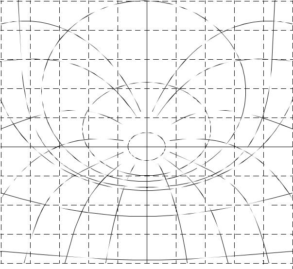
39.9 NICHOLS CHART
- a plot of the gain vs. the angle of a system transfer function after a phasor trans-
form.
• The basic method is,
1.Write an expression for the closed loop gain Gc(s)G(s).
2.Apply a phasor transform to find the gain and phase angle.
3.Gain and phase values are calculated for a large range of frequencies and plotted on the following paper.
4.Measure the gain and phase margins from the plot.
input output equations - 39.13
|
|
|
|
|
|
|
|
|
|
|
0dB |
25 |
|
|
|
|
|
|
|
0.5dB |
|
|
|
|
|
-355° |
|
|
|
|
|
|
-5° |
|
|
|
|
|
|
|
|
|
|
|
|
||
20 |
|
|
|
|
|
|
|
|
|
|
|
15 |
|
-350° |
|
|
|
|
|
|
|
-10° |
|
|
|
|
|
|
|
|
|
|
|
||
|
|
|
|
|
|
|
|
|
|
|
|
|
|
|
|
|
|
3dB |
|
|
|
|
|
10 |
|
|
|
|
|
|
|
|
|
|
|
|
|
|
|
|
|
|
|
|
|
|
-1dB |
5 |
-330° |
|
|
|
|
|
|
|
|
|
|
dB |
|
|
|
|
|
|
|
|
|
|
|
0 |
|
|
|
|
|
|
|
|
|
|
|
|
|
-300° |
|
|
|
|
|
|
|
|
|
-5 |
|
|
|
|
|
|
|
|
|
|
|
-10 |
|
|
|
|
|
|
|
|
|
-9dB |
|
|
-270° |
|
|
|
|
|
|
|
|
|
|
|
|
|
|
|
|
|
|
|
-90° |
|
|
|
|
|
|
|
|
|
|
|
|
|
|
-15 |
|
|
|
-240° |
|
|
|
|
-120° |
|
|
|
|
|
|
-210° |
-180° |
-150° |
|
|
|||
|
|
|
|
|
|
-18dB |
|
||||
|
|
|
|
|
|
|
|
|
|
|
|
-20 |
|
|
|
|
|
|
|
|
|
|
|
-280 |
-260 |
-240 |
-220 |
-200 |
-180 |
-160 |
-140 |
-120 |
-100 |
-80 |
|
|
|
|
|
|
|
phase (deg) |
|
|
|
|
|
|
|
• The gain and phase margins are measured from the plot as shown below, |
|
||||||||

input output equations - 39.14
180° |
|
|
φ |
M |
|
|
|
0dB |
GM |
|
|
|
Where, |
|
|
φ |
M = phase margin |
|
GM = gain margin |
|
•These correlate to values on the Bode plot. To find the approximate gain/phase margins with a Bode plot, locate the point where the gain is 180° to find the gain margin, and find the phase margin where the gain is 0dB.
•In unstable systems the function will circle the center point of the plot.
•
39.10BESSEL POLYNOMIALS
-put in root locus chapter?
-The following table of functions provides polynomial roots normalized to a motion that is complete in 1second [How, 2001].

input output equations - 39.15
polynomial |
roots |
order |
|
|
|
1 |
-4.6200 |
2 |
-4.0530±2.3400j |
3 |
-5.0093,-3.9668±3.7845j |
4 |
-4.0156±5.0723j,-5.5281±1.6553j |
5 |
-6.4480,-4.1104±6.3142j,-5.9268±3.0813j |
6 |
-4.2169±7.5300j,-6.2613±4.4018j,-7.1205±1.4540j |
7 |
-8.0271,-4.3361±8.7519j, -6.5714±5.6786j,-7.6824±2.8081j |
8 |
-4.4554±9.9715j,-6.8554±6.9278j,-8.1682±4.1057j,-8.7693±1.3616j |
9 |
-9.6585,-4.5696±11.1838j,-7.1145±8.1557j,-8.5692±5.3655j,-9.4013±2.6655j |
10 |
-4.6835±12.4033,-7.3609±9.3777j,-8.9898±6.6057j,-9.9657±3.9342j,- |
|
10.4278±1.3071j |
|
|
-the roots are used to construct the charateristic equation of the system.
-To increase, or decrease the reposnse time the root values are multiplied by the desired settling time.
39.11ITAE
-The Integral of Time Absolute Error (ITAE) integral equation becomes large for errors that persist for a long time.
∞
JITAE = ∫ t e( t) dt
0
- is used to select poles to minimize the integral value when selecting a characteristics equation.