

differential equations - 3.23
3.3.2 Second-order
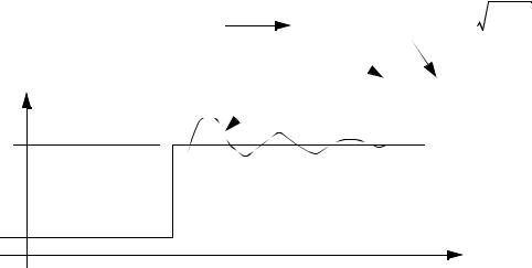
A second-order system response typically contains two first-order responses, or a first-order response and a sinusoidal component. A typical sinusoidal second-order response is shown in Figure 3.21. Notice that the coefficients of the differential equation include a damping coefficient and a natural frequency. These can be used to develop the final response, given the initial conditions and forcing function. Notice that the damped frequency of oscillation is the actual frequency of oscillation. The damped frequency will be lower than the natural frequency when the damping coefficient is between 0 and 1. If the damping coefficient is greater than one the damped frequency becomes negative, and the system will not oscillate because it is overdamped.
A second-order system, and a typical response to a stepped input.
·· |
ζω |
· |
2 |
|
σ |
|
= ζω |
n |
ω d = ω |
n 1 – ζ |
2 |
|||
y + 2 |
ny + ω |
ny = f( t) |
|
|
|
|||||||||
|
|
|
y( t) = y |
ss |
+ ( y |
0 |
– y |
|
) e–σ t cos ( ω |
d |
t) |
|
|
|
|
|
|
|
|
|
ss |
|
|
|
|
||||
yss |
|
|
|
|
|
|
|
|
|
|
|
|
|
|
y0 |
|
|
|
|
|
|
|
|
|
|
|
|
|
|
ω n
ξ
Natural frequency of system - Approximate frequency of control system oscillations.
Damping factor of system - If < 1 underdamped, and system will oscillate. If =1 critically damped. If > 1 overdamped, and never any oscillation (more like a first-order system). As damping factor approaches 0, the first peak becomes infinite in height.
ω d |
The actual frequency of oscillation - It is below the natural fre- |
|
|
|
quency because of the damping. |
Figure 3.21 The general form for a second-order system
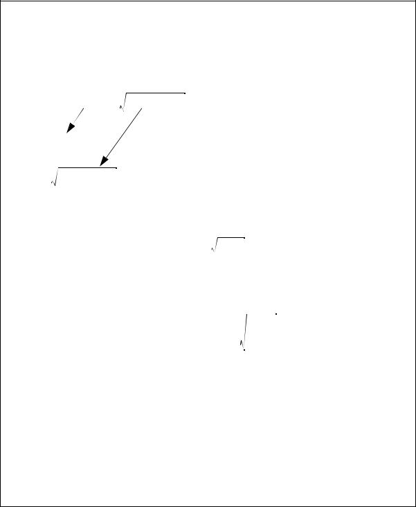
When only the damping coefficient is increased, the frequency of oscillation, and overall response time will slow, as seen in Figure 3.22. When the damping coefficient is 0 the system will oscillate indefinitely. Critical damping occurs when the damping coeffi-
differential equations - 3.24
cient is 1. At this point both roots of the differential equation are equal. The system will not oscillate if the damping coefficient is greater than or equal to 1.
ξ = 0
ξ = 0.5
(underdamped)
ξ |
1 |
= ------ = 0.707 |
|
|
2 |
ξ = 1 (critical)
(overdamped)
ξ » 1
Figure 3.22 The effect of the damping coefficient
When observing second-order systems it is more common to use more direct measurements of the response. Some of these measures are shown in Figure 3.23. The rise

differential equations - 3.25
time is the time it takes to go from 10% to 90% of the total displacement, and is comparable to a first order time constant. The settling time indicates how long it takes for the system to pass within a tolerance band around the final value. The permissible zone shown is 2%, but if it were larger the system would have a shorter settling time. The period of oscillation can be measured directly as the time between peaks of the oscillation, the inverse is the damping frequency. (Note: don’t forget to convert to radians.) The damped frequency can also be found using the time to the first peak, as half the period. The overshoot is the height of the first peak. Using the time to the first peak, and the overshoot the damping coefficient can be found.
|
|
|
|
|
|
|
|
|
|
|
|
|
|
|
|
|
|
|
|
|
|
|
|
|
|
|
|
|
|
|
|
|
|
|
|
|
|
|
|
|
Note: This figure is not to scale to make details |
||||||||||||||||||||||||||||||||||||||||||||||||||||
|
|
|
|
|
|
|
|
|
|
|
|
|
|
|
|
tp |
|
|
|
|
|
|
|
|
|
|
|
1 |
|
|
|
|
|
|
near the steady-state value easier to see. |
||||||||||||||||||||||||||||||||||||||||||||||||||||||||||
|
|
|
|
|
|
|
|
|
|
|
|
|
|
|
|
|
|
|
|
|
|
|
|
|
|
|
|
|
|
|
|
|
|||||||||||||||||||||||||||||||||||||||||||||||||||||||||||||
|
|
|
|
|
|
|
|
|
|
|
|
|
|
|
|
|
|
|
|
|
|
|
|
|
|
|
|
|
|
|
|
|
|
|
|
|
|
|
|
|
|
|
|
|
|
|
|
|
|
|
|
|
|
|
|
|
|
|
|
|
|
|
|
|
|
|
|
|
|
|
|
|
|
|
|
|
|
|
|
|
|
|
|||||||||||
|
|
|
|
|
|
|
|
|
|
|
|
|
|
|
|
|
|
|
|
|
|
|
|
|
|
|
|
|
|
|
|
|
|
|
|
|
|
|
|
|
|
|
|
|
|
|
|
|
|
|
|
|
|
|
|
|
|
|
|
|
|
|
|
|
|
|
|
|
|
|
|
|
|
|
|
|
|
|
|
|
|
|
|||||||||||
|
|
|
|
|
|
|
|
|
|
|
|
|
|
|
|
|
|
|
|
|
|
|
|
|
|
|
|
f |
d |
= |
-- |
|
|
|
T |
|
|
|
|
|
|
|
|
|
|
|
|
|
|
|
|
|
|
|
|
|
|
|
|
|
|
|
|
|
|
|
|
|
|
|
|
|
|
|
|
|
|
|
|
|
|
|
|
|
|
||||||||
|
|
|
|
|
|
|
|
|
|
|
|
|
|
|
|
|
|
|
|
|
|
|
|
|
|
|
|
|
|
|
|
|
|
T |
|
|
|
|
|
|
|
|
|
|
|
|
|
|
|
|
|
|
|
|
|
|
|
|
|
|
|
|
|
|
|
|
|
|
|
|
|
|
|
|
|
|
|
|
|
|
|
ess |
|||||||||||
|
|
|
|
|
|
|
|
|
|
|
|
|
|
|
|
|
|
|
|
|
|
|
|
|
|
|
|
|
|
|
|
|
|
|
|
|
|
|
|
|
|
|
|
|
|
|
|
|
|
|
|
|
|
|
|
|
|
|
|
|
|
|
|
|
|
|
|
|
|
|
|
|
|
|
|
|
|
|
|
|
|||||||||||||
|
|
|
|
|
|
|
|
|
|
|
|
|
|
|
|
|
|
|
|
|
|
|
|
|
|
|
|
|
|
|
|
|
|
|
|
|
|
|
|
|
|
|
|
|
|
|
|
|
|
|
|
|
|
|
|
|
|
|
|
|
|
|
|
|
|
|
|
|
|
|
|
|
|
|
|
|
|
|
|
|
|
|
|
|
|
|
|
|
|
|
|||
|
|
|
|
|
|
|
|
|
|
|
|
|
|
|
|
|
|
|
|
|
|
|
|
|
|
|
|
|
|
|
|
|
|
|
|
|
|
|
|
|
|
|
|
|
|
|
|
|
|
|
|
|
|
|
|
|
|
|
|
|
|
|
|
|
|
|
|
|
|
|
|
|
|
|
|
|
|
|
|
|
|
|
|
|
|
|
|
||||||
|
|
0.02∆ x |
|
|
|
|
|
|
|
|
|
|
|
|
|
|
|
|
|
|
|
|
|
|
|
|
|
|
|
|
|
|
|
|
|
|
|
|
|
|
|
|
|
|
|
|
|
|
|
|
|
|
|
|
|
|
|
|
|
|
|
|
|
|
|
|
|
|
|
|
|
|
|
|
|
|
|
|
|
|
|
|
|
|
|
||||||||
|
|
|
|
|
|
|
|
|
|
|
|
|
|
b |
|
|
|
|
|
|
|
|
|
|
|
|
|
|
|
|
|
|
|
|
|
|
|
|
|
|
|
|
|
|
|
|
|
|
|
|
|
|
|
|
|
|
|
|
|
|
|
|
|
|
|
|
|
|
|
|
|
|
|
|
|
|
|
|
|
|
|
|
|
|
|
|
|||||||
|
|
|
|
|
|
|
|
|
|
|
|
|
|
|
|
|
|
|
|
|
|
|
|
|
|
|
|
|
|
|
|
|
|
|
|
|
|
|
|
|
|
|
|
|
|
|
|
|
|
|
|
|
|
|
|
|
|
|
|
|
|
|
|
|
|
|
|
|
|
|
|
|
|
|
|
|
|
|
|
|
|
|
|
|
|
||||||||
|
|
|
|
|
|
|
|
|
|
|
|
|
|
|
|
|
|
|
|
|
|
|
|
|
|
|
|
|
|
|
|
|
|
|
|
|
|
|
|
|
|
|
|
|
|
|
|
|
|
|
|
|
|
|
|
|
|
|
|
|
|
|
|
|
|
|
|
|
|
|
|
|
|
|
|
|
|
|
|
|
|
||||||||||||
|
|
|
|
|
|
|
|
|
|
|
|
|
|
|
|
|
|
|
|
|
|
|
|
|
|
|
|
|
|
|
|
|
|
|
|
|
|
|
|
|
|
|
|
|
|
|
|
|
|
|
|
|
|
|
|
|
|
|
|
|
|
|
|
|
|
|
|
|
|
|
|
|
|
|
|
|
|
|
|
|
|
|
|
||||||||||
|
|
|
|
|
|
|
|
|
|
|
|
|
|
|
|
|
|
|
|
|
|
|
|
|
|
|
|
|
|
|
|
|
|
|
|
|
|
|
|
|
|
|
|
|
|
|
|
|
|
|
|
|
|
|
|
|
|
|
|
|
|
|
|
|
|
|
|
|
|
|
|
|
|
|
|
|
|
|
|
|
|
|
|
|
|
|
|
|
|
|
|
|
|
|
|
0.02∆ x |
|
|
|
|
|
|
|
|
|
|
|
|
|
|
|
|
|
|
|
|
|
|
|
|
|
|
|
|
|
|
|
|
|
|
|
|
|
|
|
|
|
|
|
|
|
|
|
|
|
|
|
|
|
|
|
|
|
|
|
|
|
|
|
|
|
|
|
|
|
|
|
|
|
|
|
|
|
|
|
|
|
|
|
|
|
|
|
|
|
||
|
|
|
|
|
|
|
|
|
|
|
|
|
|
|
|
|
|
|
|
|
|
|
|
|
|
|
|
|
|
|
|
|
|
|
|
|
|
|
|
|
|
|
|
|
|
|
|
|
|
|
|
|
|
|
|
|
|
|
|
|
|
|
|
|
|
|
|
|
|
|
|
|
|
|
|
|
|
|
|
|
|
|
|
|
|
|
|
|
|
|
|||
|
|
|
|
|
|
|
|
|
|
|
|
|
|
|
|
|
|
|
|
|
|
|
|
|
|
|
|
|
|
|
|
|
|
|
|
|
|
|
|
|
|
|
|
|
|
|
|
|
|
|
|
|
|
|
|
|
|
|
|
|
|
|
|
|
|
|
|
|
|
|
|
|
|
|
|
|
|
|
|
|
|
|
|
|
|
|
|
|
|
||||
|
|
|
|
|
|
|
|
|
|
|
|
|
|
|
|
|
|
|
|
|
|
|
|
|
|
|
|
|
|
|
|
|
|
|
|
|
|
|
|
|
|
|
|
|
|
|
|
|
|
|
|
|
|
|
|
|
|
|
|
|
|
|
|
|
|
|
|
|
|
|
|
|
|
|
|
|
|
|
|
|
|
|
|
|
|
|
|
|
|
||||
|
|
|
|
|
|
|
|
|
|
|
|
|
|
|
|
|
|
|
|
|
|
|
|
|
|
|
|
|
|
|
|
|
|
|
|
|
|
|
|
|
|
|
|
|
|
|
|
|
|
|
|
|
|
|
|
|
|
|
|
|
|
|
|
|
|
|
|
|
|
|
|
|
|
|
|
|
|
|
|
|
|
|
|
|
|
|
|
|
|||||
|
|
|
|
|
|
|
|
|
|
|
|
|
|
|
|
|
|
|
|
|
|
|
|
|
|
|
|
|
|
|
|
|
|
|
|
|
|
|
|
|
|
|
|
|
|
|
|
|
|
|
|
|
|
|
|
|
|
|
|
|
|
|
|
|
|
|
|
|
|
|
|
|
|
|
|
|
|
|
|
|
|
|
|
|
|
|
|
|
|
|
|
|
|
|
|
|
|
|
|
|
|
|
|
|
|
|
|
|
|
|
|
|
|
|
|
|
|
|
|
|
|
|
|
|
|
|
|
|
|
|
|
|
|
|
|
|
|
|
|
|
|
|
|
|
|
|
|
|
|
|
|
|
|
|
|
|
|
|
|
|
|
|
|
|
|
|
|
|
|
|
|
|
|
|
|
|
|
|
|
|
|
|
|
|
|||
|
|
0.9∆ x |
|
|
|
|
|
|
|
|
|
|
|
|
|
|
|
|
|
|
|
|
|
|
|
|
|
|
|
|
|
|
|
|
|
|
|
|
|
|
|
where, |
|
|
|
|
|
|
|
|
|
|
|
|
|
|
|
|
|
|
|
|
|
|
|
|
|
|
|
|
|
|
|
|
|
|
|
|
|
|
|
|
|
||||||||||
|
|
|
|
|
|
|
|
tr |
|
|
|
|
|
|
|
|
|
|
|
|
|
ts |
|
|
|
|
|
|
|
|
|
|
|
|
|
|
|
|
|
|
|
|
|
|
|
|
|
|
|
|
|
|
|
|
|
|
|
|
|
|
|
|
|
|
|
|
|
|
|
|
|
|
|
|
|||||||||||||||||||
|
|
|
|
|
|
|
|
|
|
|
|
|
|
|
|
|
|
|
|
|
|
|
|
|
|
|
|
|
|
|
|
|
|
|
|
|
|
|
|
|
|
|
|
|
|
|
|
|
|
|
|
|
|
|
|
|
|
|
|
|
|
|
|
|
|
|
|
|
|
|
|
|
|
|
|
||||||||||||||||||
∆ x |
|
|
|
|
|
|
|
|
|
|
|
|
|
|
|
|
|
|
|
|
|
|
|
|
|
|
|
|
|
|
|
|
|
|
|
|
|
|
|
|
|
|
|
|
|
|
|
tr = rise time (from 10% to 90%) |
|||||||||||||||||||||||||||||||||||||||||||||
|
|
|
|
|
|
|
|
|
|
|
|
|
|
|
|
|
|
|
|
|
|
|
|
|
|
|
|
|
|
|
|
|
|
|
|
|
|
|
|
|
|
|
|
|
|
|
ts |
= |
|
settling time (to within 2-5% typ.) |
|||||||||||||||||||||||||||||||||||||||||||
|
|
|
|
|
|
|
|
|
|
|
|
|
|
|
|
|
|
|
|
|
|
|
|
|
|
|
|
|
|
|
|
|
|
|
|
|
|
|
|
|
|
|
|
|
|
|
|
|
∆ x |
= |
|
|
|
total displacement |
|||||||||||||||||||||||||||||||||||||||
|
|
0.5∆ x |
|
|
|
|
|
|
|
|
|
|
|
|
|
|
|
|
|
|
|
|
|
|
|
|
|
|
|
|
|
|
|
|
|
|
|
|
|
|
|
|
|
|
|
|
|
||||||||||||||||||||||||||||||||||||||||||||||
|
|
|
|
|
|
|
|
|
|
|
|
|
|
|
|
|
|
|
|
|
|
|
|
|
|
|
|
|
|
|
|
|
|
|
|
|
|
|
|
|
|
|
T, fd = period and frequency - damped |
||||||||||||||||||||||||||||||||||||||||||||||||||
|
|
|
|
|
|
|
|
|
|
|
|
|
|
|
|
|
|
|
|
|
|
|
|
|
|
|
|
|
|
|
|
|
|
|
|
|
|
|
|
|
|
|
|
|
|
|
|
||||||||||||||||||||||||||||||||||||||||||||||
|
|
0.1∆ x |
|
|
|
|
|
|
|
|
|
|
|
|
|
|
|
|
|
|
|
|
|
|
|
|
|
|
|
|
|
|
|
|
|
|
|
|
|
|
|
|
|
|
b = overshoot |
|
|
|
|
|
|
|
|
|
|
|
|
|
|
|
|
|
|
|
|
||||||||||||||||||||||||||||
|
|
|
|
|
|
|
|
|
|
|
|
|
|
|
|
|
|
|
|
|
|
|
|
|
|
|
|
|
|
|
|
|
|
|
|
|
|
|
|
|
|
|
|
|
|
|
|
|
|
|
|
|
|
|
|
|
|
|
|
|
|
|
|
||||||||||||||||||||||||||||||
|
|
|
|
|
|
|
|
|
|
|
|
|
|
|
|
|
|
|
|
|
|
|
|
|
|
|
|
|
|
|
|
|
|
|
|
|
|
|
|
|
|
|
|
tp |
= |
|
|
time to first peak |
|
|
|
|
|
|
|
|
|
|
|
|
|
|
|
|
|
|
|
|
|||||||||||||||||||||||||
|
|
|
|
|
|
|
|
|
|
|
|
|
|
|
|
|
|
|
|
|
|
|
|
|
|
|
|
|
|
|
|
|
|
|
|
|
|
|
|
|
|
|
|
|
|
|
|
|
|
|
|
|
|
|
|
|
|
|
|
|
|
|
|
|
|
|
|
|
|
|
|||||||||||||||||||||||
|
|
|
|
|
|
|
|
|
|
|
|
|
|
|
|
|
|
|
|
|
|
|
|
|
|
|
|
|
|
|
|
|
|
|
|
|
|
|
|
|
|
|
|
|
|
|
|
|
ess |
= |
|
|
|
steady state error |
|||||||||||||||||||||||||||||||||||||||
|
|
|
|
|
|
|
|
|
|
|
|
|
|
|
|
|
|
|
|
|
|
|
|
|
|
|
|
|
|
|
|
|
|
|
|
|
|
|
|
|
|
|
|
|
|
||||||||||||||||||||||||||||||||||||||||||||||||
|
|
|
|
|
|
|
|
|
|
|
|
|
|
|
|
|
|
|
|
|
|
|
|
|
|
|
|
|
|
–σ t |
|
|
|
|
|
|
|
|
|
|
|
|
|
|
ω |
|
|
|
≈ |
|
π |
|
|
|
|
|
|
|
|
(1) |
|
|
|
|
|
|
|
|
|
|
|
|
|
|
|
||||||||||||||||||
|
|
|
|
|
|
|
|
|
|
|
|
|
|
|
|
|
|
|
|
|
|
|
|
|
|
|
|
|
|
|
|
|
|
|
|
|
|
|
|
|
|
|
|
|
|
|
|
|
|
|
|
|
|
|
|
|
|
|
|
|
|
|
|
|
|
|
|
|
|
||||||||||||||||||||||||
|
|
|
|
|
|
|
|
|
|
|
|
|
|
|
|
|
|
|
|
|
|
x |
|
|
|
|
|
|
cos ( ω |
|
dt) |
|
|
|
|
|
d |
|
---- |
|
|
|
|
|
|
|
|
|
|
|
|
|
|
|
|
|
|
|
|
|
|
|
|
|
|
|
|||||||||||||||||||||||||||
|
|
|
|
|
|
|
|
|
|
|
|
|
|
|
|
|
|
|
|
|
|
= ∆ xe |
|
|
|
|
|
|
|
|
|
|
|
|
|
|
|
t |
p |
|
|
|
|
|
|
|
|
|
|
|
|
|
|
|
|
|
|
|
|
|
|
|
|
|
|
|
|
||||||||||||||||||||||||||
|
|
|
|
|
|
|
|
|
|
|
|
|
|
|
|
|
|
|
|
|
|
|
|
|
|
|
|
|
|
|
|
|
|
|
|
|
|
|
|
|
|
|
|
|
|
|
|
|
|
|
|
|
|
|
|
|
|
|
|
|
|
|
|
|
|
|
|
|
|
|
|
|
|
|
|
|
|
|
|
|
|
|
|
|
|
|
|||||||
|
|
|
|
|
|
|
|
|
|
|
|
|
|
|
|
|
|
|
|
|
|
|
|
|
|
|
|
|
|
|
|
|
|
|
|
|
|
|
|
|
|
|
|
|
|
|
|
|
σ |
|
|
= ξω |
|
|
n |
|
|
|
|
|
|
|
|
(2) |
|
|
|
|
|
|
|
|
|
|
|
|
|
|
|
||||||||||||||
|
|
|
|
|
|
|
|
|
|
|
|
|
|
|
|
|
|
|
|
|
|
|
|
|
|
|
|
|
|
|
|
|
|
|
|
|
|
|
|
|
|
|
|
|
|
|
|
|
b |
= |
|
|
|
|
–σ tp |
|
|
|
|
|
|
|
|
(3) |
|
|
|
|
|
|
|
|
|
|
|
|
|
|
|
||||||||||||||
|
|
|
|
|
|
|
|
|
|
|
|
|
|
|
|
|
|
|
|
|
|
|
|
|
|
|
|
|
|
|
|
|
|
|
|
|
|
|
|
|
|
|
|
------ |
|
|
|
e |
|
|
|
|
|
|
|
|
|
|
|
|
|
|
|
|
|
|
|
|
|
|
|
||||||||||||||||||||||
|
|
|
|
|
|
|
|
|
|
|
|
|
|
|
|
|
|
|
|
|
|
|
|
|
|
|
|
|
|
|
|
|
|
|
|
|
|
|
|
|
|
|
|
|
|
|
|
|
∆ x |
= |
|
|
|
|
1 |
|
|
|
|
|
|
|
|
|
|
|
|
|
|
|
|
|
|
|
|
|
|
|
|
|
|
|
|
||||||||||
|
|
|
|
|
|
|
|
|
|
|
|
|
|
|
|
|
|
|
|
|
|
|
|
|
|
|
|
|
|
|
|
|
|
|
|
|
|
|
|
|
|
|
|
|
|
|
|
|
ξ |
|
|
|
----------------------------- |
|
|
|
|
(4) |
|
|
|
|
|
|
|
|
|
|
|
|
|
|
|
||||||||||||||||||||
|
|
|
|
|
|
|
|
|
|
|
|
|
|
|
|
|
|
|
|
|
|
|
|
|
|
|
|
|
|
|
|
|
|
|
|
|
|
|
|
|
|
|
|
|
|
|
|
|
|
|
|
|
|
|
|
|
|
|
|
|
π |
2 |
|
|
|
|
|
|
|
|
|
|
|
|
|
|
|
|
|
|
|
|
|
||||||||||
|
|
|
|
|
|
|
|
|
|
|
|
|
|
|
|
|
|
|
|
|
|
|
|
|
|
|
|
|
|
|
|
|
|
|
|
|
|
|
|
|
|
|
|
|
|
|
|
|
|
|
|
|
|
|
|
|
|
|
|
|
|
|
|
|
|
|
|
|
|
|
|
|
|
|
|
|
|
|
|
|
|
|
|
|
|
|
|||||||
|
|
|
|
|
|
|
|
|
|
|
|
|
|
|
|
|
|
|
|
|
|
|
|
|
|
|
|
|
|
|
|
|
|
|
|
|
|
|
|
|
|
|
|
|
|
|
|
|
|
|
|
|
|
|
|
|
|
|
|
------- |
|
+ 1 |
|
|
|
|
|
|
|
|
|
|
|
|
|
|
|
|
|
|
|
|
|
|
|
|
|||||||
|
|
|
|
|
|
|
|
|
|
|
|
|
|
|
|
|
|
|
|
|
|
|
|
|
|
|
|
|
|
|
|
|
|
|
|
|
|
|
|
|
|
|
|
|
|
|
|
|
|
|
|
|
|
|
|
|
|
|
|
|
tpσ |
|
|
|
|
|
|
|
|
|
|
|
|
|
|
|
|
|
|
|
|
|
|
|
|
|
|
|
|
||||
Figure 3.23 Characterizing a second-order response (not to scale)
differential equations - 3.26
Note: We can calculate these relationships using the complex homogenous form, and the generic second order equation form.
A2 + 2ξω nA + ω n2 = 0 |
|
|
|
|
|
|
|
|
||||||||||
A |
= |
– 2ξω |
n |
± |
4ξ 2ω n2 – 4ω |
n2 |
= σ ± |
jω d |
|
|
|
|
|
|||||
----------------------------------------------------------- |
|
|
|
|
|
|||||||||||||
|
|
|
|
|
|
|
|
|
2 |
|
|
|
|
|
|
|
|
|
–2ξω |
n |
= |
σ |
= |
–ξω |
n |
|
|
ω |
n = |
σ |
(1) |
||||||
--------------- |
|
|
----- |
|||||||||||||||
|
|
2 |
|
|
|
|
|
|
|
|
|
|
|
|
|
|
–ξ |
|
|
4ξ 2ω |
n2 – 4ω |
n2 |
= jω |
d |
|
|
|
|
|
|
|
|
|||||
----------------------------------- |
|
|
|
|
|
|
|
|
||||||||||
|
|
|
|
2 |
|
|
|
|
|
|
|
|
|
|
|
|
|
|
4ξ 2ω n2 – 4ω n2 = 4( –1)ω d2 |
|
|
|
|
|
|
|
|
||||||||||
ω |
2 |
– |
ξ |
2 |
ω |
2 |
= |
ω |
2 |
|
|
ω n 1 – ξ |
2 |
= |
ω d |
(2) |
||
n |
|
n |
d |
|
|
|
|
|||||||||||
σ |
2 |
– ξ |
2 |
σ |
2 |
= |
ω |
2 |
|
|
|
|
|
|
|
|
|
|
----- |
|
----- |
d |
|
|
|
|
|
|
|
|
|
||||||
ξ |
2 |
|
|
|
ξ |
2 |
|
|
|
|
|
|
|
|
|
1 |
|
|
1 |
|
|
ω |
d |
|
|
|
|
|
|
ξ |
= |
|
|
|
|
||
|
|
|
|
|
|
|
|
------------------- |
|
|||||||||
|
|
|
|
|
2 |
|
|
|
|
|
|
|
|
(3) |
||||
---- |
= |
|
----- |
+ 1 |
|
|
|
|
|
|
|
ω |
2 |
|
||||
ξ |
2 |
|
|
σ |
2 |
|
|
|
|
|
|
|
|
|
d |
+ 1 |
|
|
|
|
|
|
|
|
|
|
|
|
|
|
|
σ |
2 |
|
|||
|
|
|
|
|
|
|
|
|
|
|
|
|
|
|
----- |
|
|
|
The time to the first peak can be used to find the approximate decay constant
x( t) |
= C |
1 |
e–σ t cos ( ω |
d |
t + C ) |
|||
|
|
|
|
|
2 |
|||
ω |
d = |
π |
|
|
|
|
|
|
--- |
|
|
|
|
|
|
||
|
|
tp |
|
|
|
|
|
|
b ≈ ∆ xe–σ tp ( 1) |
|
|
||||||
|
|
ln |
|
|
b |
|
|
|
|
|
|
----- |
|
|
|||
σ |
= |
|
∆ x |
|
|
|||
–----------------- |
|
|
||||||
|
|
|
|
tp |
|
|
||
(4)
(5)
Figure 3.24 Second order relationships between damped and natural frequency

differential equations - 3.27
2.2 |
|
|
y(t) |
2.0 |
|
|
t |
0 |
5.0 |
4.0 |
Write a function of time for the graph. (Note: measure, using a ruler, to get values.) Find the natural frequency and damping coefficient to develop the differential equation. Using the dashed lines determine the settling time.
ans. |
|
|
|
|
t < |
4 |
y( t) |
= |
0 |
t ≥ |
4 |
y( t) |
= |
|
Figure 3.25 Drill problem: Find the equation given the response curve