Сборник трудов конференции СПбГАСУ 2012

Численные методы расчетов в практической геотехнике

4. Simulation of the Construction of the Central Tower

The construction of the central tower can be divided into three steps: (1) earth fill construction, (2)lower structure of the central tower, and (3) the subtowers and the upper structure of the central tower. Steps (2) and (3) correspond to Part I and Part II in Fig. 7.

Load(kPa)

Fig. 7. Two steps for Bayon construction

5.Analysis Result

Fig. 6 shows equi-settlement contour lines of the soil foundation after the loads of the two steps have been applied. The result of this calculation was a settlement of around 12cm at the center of the main tower, 10cmat the edges ofthe main tower, and around 7 to 8 cm around the periphery of the subtowers.

Fig. 9 shows measured heights at the north-south crossroad of the main tower. It is clear from this figure that in both of the north-south and east-west sections, the heightofthecentralareaisnotnecessarilylowerthanitsperiphery.Wedidnotscrutinize this point in detail, since it is unclear how the height of the foundation was established in the first place, at the time of construction of the central tower.

6. Simulation of the Excavation inside the Main Chamber of the Central Tower

In 1933, a roughly 14m-deep shaft was dug in the center of the main chamber and backfilled, but the backfill was not compacted. To examine this condition, we excavateda2m-diametershaftinthecentralareafromthegroundsurfaceandobserved changes in stress.

Yoshinori Iwasaki

Fig. 8. Equi-settlement contour lines in soil foundation after completion of Bayon Tower

Fig. 9 Height of the base mound for the

Central Tower S-N and W-E sections

Численные методы расчетов в практической геотехнике

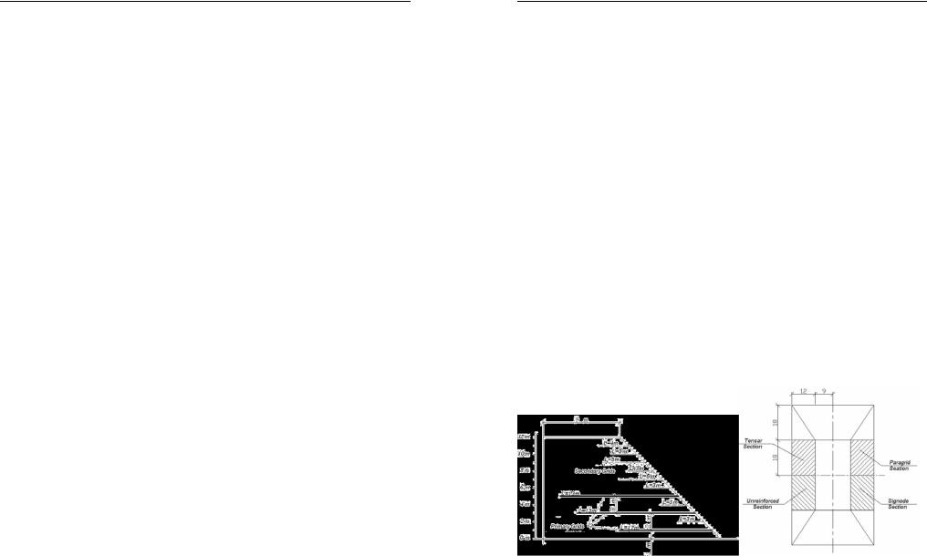
σFig. 11 shows changes in stress around the v shaftbeforeand aftershaftexcavationatlevel from GL+10m to +11m directly beneath the foundation.

surface, or radial stress, became zero at the boundary of the shaft. This is because the airpressurewasappliedtotheexcavatedsurfacesothatradialstresspracticallybecame zero at a radius of 1m.

Fig. 11. Change of stress by shaft excavation at level GL;10-11m

However, radial stress increased with greater distance from the shaft surface due to cohesion and the internal angle of friction and peakedatr=4m,butdecreasedatdistancesover 4m.

Tangential stress runs perpendicular to radialstress. Itinducesa compressive stressin the shape of a ring around the shaft, maximum

Fig. 12. Stress state around shaft ring stress occurred near r=2m at the height of the ground level.

Yoshinori Iwasaki

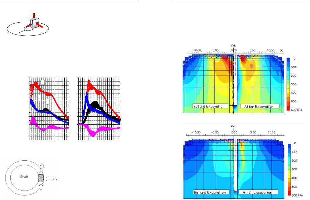
The stability issue around the axi-symmetric shaft cavity can be explained in terms of shear failure caused by differential stress between tangential and radial stress inthe ringofground,asshowninFig.12.Ifshear strengthissufficientlylarge,tangential stressbecomeslargest at the shaftsurfaceand then decreasesas the radius increases. If shear strength is small, a failure occurs, and the stress also decreases in strength.

AsshowninFig.13,tangentialstresswaslargerthanshearstrengthbetweenr=1m andr=2m,sostressredistributionoccurredanddecreasedshearstress.Thismeansthatthe stress ringoccurred near r = 2 m, and the area inside r = 2mwasa stress-free zone.

Fig. 13. Change of vertical stress(σv) in the foundation mound by vertical shaft

Fig. 14. Change of tangential stress(σθ) in the foundation mound by vertical shaft

Численные методы расчетов в практической геотехнике

Figs. 13 and 14 showstress distribution in the platform ground before and after shaft excavation. Fig. 13 shows changes in vertical stress and Fig. 14 shows changes in tangentialstress.Vertical stresswaszero atthegroundsurface in the center of the platform before shaft excavation, and the formationofaconicalstresswedgeprovidedstability,butafter shaft excavation, the center of the wedge disappeared, and a concentration of vertical stress occurred directly beneath the elliptical foundation inside the main chamber.

The sandy soil of Angkor is strong when it is dry, but becomes weak in wet condition. Because strength decreases in times of flood, this condition becomes dangerous from a broad perspective.

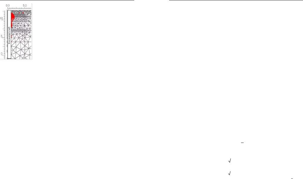
Fig. 15 shows the estimated plastic range of the ground around the shaft. It is subject to change according to the strength conditions (Table-1)that areinitiallyset. In other words, if strengthincreases,

the plastic range shrinks, and if strength decreases, the plastic range expands.

7. Conclusion

It is surprising that the chamber existed on hollow ground without collapsing for some 75 years since the 1933 excavation, although the sitting Buddha statue was buried even way before that. Rainfall from the top of the tower is not completely blocked, but it seems that when a plastic range was formed around the cavity, a large confining stress created by the concentration of vertical pressure near a distance of 2.5 m from the center prevented the expansion of the plastic region and helped maintain stability. However, if rainwater seeps into the earth fill around the cavity, the chamberwouldcollapse.Toprovidepermanentstability,suchmeasuresasre-excavation of the shaft to compact the loose fill of the pit as well as applying a lining.

T. Tanaka (The JapanAssociation of Rural Solutions for Environmental Conservation and Resource Recycling (JARUS), Tokyo, Japan)

M. Ariyosh, Y. Mohri (National Institute for Rural Engineering, Tsukuba, Japan)

DISPLACEMENT, STRESSAND STRAIN OFFLEXIBLEBURIED PIPE TAKINGINTOACCOUNTTHE CONSTRUCTION PROCESS

There are few suitable studies concerning the deformation analysis of a large scale flexible pipe that is taking into account the construction process with a complex earth pressure condition. In this study we attempted to clarify the deformation, stress

282

T. Tanaka, M. Ariyosh, Y. Mohri

andstrainofpipebythefiniteelementanalysiswithimplicit-explicitdynamicrelaxation method. By comparing theresults of real scale field experiment with those of the finite elementanalysis,weestimatedthepossibilityofthefiniteelementanalysisforprediction of deormation, stress and strain of large scale buried pipe. The displacement and stress by the finite element analysis agreed well to those of field experiment.

1.INTRODUCTION

This paper presents deformation, stress and strain of a large scale flexible pipe that is taking into account the construction process: excavation and back-filling. It seemsimportanttodevelopanumericalmethodforanalyzingsuchcomplexinteractive action of soils and flexible structure. The problem was attempted to solve by elastoplastic finite element analysis with implicit-explicit dynamic relaxation method. Field experiments were carried out by measuring the deflections and strains of steel pipe, then mechanical properties of soils were determined by triaxial tests. Comparing the resultsoftheanalysisandtheexperiment,thereliabilityofthedevelopedelasto-plastic analysis with construction process was evaluated.

2.MATERAILMODEL

A material model for a real granular material was used with the features of nonlinearpre-peak,pressure-sensitivityofthedeformationand strengthcharacteristics of sand, non-associated flow characteristics, post-peak strain softening, and strainlocalization into a shearband with aspecific width (Tatsuokaetal., 1991; Siddiqueeet al., 1999). The material model is briefly described in this section.

The yield function ( f ) and the plastic potential function (Ф) are given by;

where I1 is the first invariant (positive in tension) of deviatoric stresses and σ is the

second invariant of deviatoric stress. With the Mohr-Coulomb model, g(θL ) takes the following form;

283

Численные методы расчетов в практической геотехнике

φ is the mobilized friction angle andθL is the Lode angle. The frictional hardeningsoftening functions expressed as follows were used;

where m, ε f and εr are the materialconstantsand α p and αr are the valuesof α at the peak and residual states.

The residual friction angle (φr ) and Poissons ratio (ν ) werechosen based on the

data from the test of air-dried dense Toyoura sand. The elastic moduli are estimated using the following equations.

Thepeakfrictionangle(φP )wasestimatedfromthefollowingempiricalrelations

based on the plane strain compression test on dense Toyoura sand.

The peak friction angle is a function of confining pressure, initial void ratio e and angle δ of the direction of major principal stress σ1 relative to the horizontal

bedding plane. The dilatancy angle (ψ ) was estimated from Rowes stress-dilatancy relation.

The introduction of shear banding in the numerical analysis was achieved by introducing a strain localization parameter s in the following additive decomposition of total strain increment as follows;

3. FINITE ELEMENTANALYSIS

The finite element used in this study is a pseudo-equilibrium model by one-point integration of a 4-noded Lagrange-type element. The implicit-explicit dynamic

284

T. Tanaka, M. Ariyosh, Y. Mohri

relaxation method combined with the generalized return mapping algorithmis applied to theintegration algorithms of elasto-plasticconstitutive relations includingtheeffect oftheshearbanding(TanakaandKawamoto,1988;Okajima,TanakaandMori,2001).

4.LAYERED ELEMENT

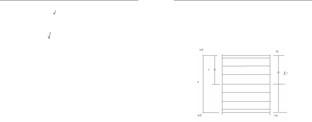
We employa layered approach based on the isoparametric 8 noded element to a steelpipe.Layersarenumberedsequentiallystartingatthebottomandlayersofdifferent thickness can be employed.

Figure 1. Layer model for a thin steel pipe based on isoparametric 8 noded element

In the formulation of stiffness matrix, strain matrix B is calculated at the mid-

where ξis a linear coordinate in the thickness direction andηare curvilinear coordinate of isoparametricelement, DistheelasticitymatrixandJ isthedeterminatoftheJacobianmatrix.

5.FIELD EXPERIMENT

Figure 2 shows the real scale field experiment of buried pipe. The soil mass (mainly loam) of the site was excavated and steel pipe (diameter: 3500 mm, pipe thickness: 24 mm, SM490) was placed. The length of pipe is 5 m. The back-filling by

285

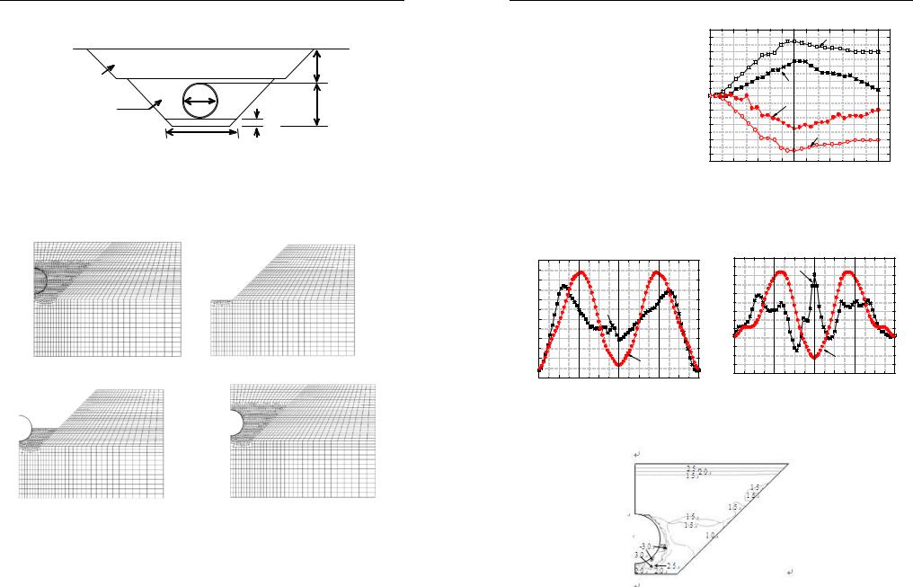
Численные методы расчетов в практической геотехнике

aggregate was accomplished with controlled 30cm layers and compacting the fill to 90 % compaction.

7406

unit:mm

Figure 2. Cross section of field experiment

The construction process of buried pipe is shown Figure 3. Initially all elements aresoilsandafterexcavationthepipewassetanddeformedbyselfweight.Thematerial constants of soils and aggregate used for analysis were obtained by triaxial test.

Figure 3. The construction process of buried pipe

The Figure 4 shows the deflections of the pipe during back-filling process. In this figure, deflection of pipe at the initial stage is set to be zero. The deflections by the analysis show similar to field test result, but the result by analysis is a little bit larger because the assumed initial horizontal stress 20kPa of each layer may be rather large.

286

Численные методы расчетов в практической геотехнике

6.CONCLUSIONS

We attempted to solve the deformation, stress and strain of flexible buried pipe bythe elasto-plastic finite element analysis that is taking into acoount the construction process. The conclusions are summarized as follows.

1.Theobserveddeflectionofthepipecanbesimulatedwellbytheelasto-plastic finiteelementanalysis.Alsotheobservedstrainofinternalsurfaceofpipewassimulated reasonably well by the analysis

2.Thecomputedstressbythefiniteelementanalysisshowedcomplexdistribution around the pipe especially the bottom back-fill soils and it is important to follow the

construction process that is taking into account the interaction of soils and structure.

References

1.Okajima,K.,Tanaka,T.andMori,H.(2001),Elasto-plasticfiniteelementcollapseanalysis of retaining wall by excavatio., Computational Mechanics New Frontiers for the New Millennium, Vol.1, 439-444.

2.Siddiquee,M.S.A.,Tanaka,T.,Tatsuoka,F.,Tani,K. andMorimoto,T.(1999), Numerical simulation of bearing capacity characteristics of strip footing on sand, Soils and Foundations, Vol. 39, No. 4, 93-109.

3.Tanaka, T. and Kawamoto, O., (1988), Three dimensional finite element collapse analysis for foundations and slopes using dynamic relaxation, in Proceedings of Numerical Methods in Geomechanics,Insbruch, 1213-1218.

4.Tatsuoka, F., Okahara, M., Tanaka, T., Tani, K., Morimoto, T. and Siddiquee, M. S. A., (1991), Progressive Failure and Particle Size Effect in Bearing Capacity of a Footing on Sand,

Geotechnical Engineering Congress -ASCE, Geotechnical Special Publication 27, Vol. 2, 788-802.

A.Zh.Zhussupbekov, R.E.Lukpanov,A.Tulebekova, I.O.Morev,Y.B.Utepov

(Geotechnical Institute of L.N. Gumilyov Eurasian National University,

Astana, Kazakhstan),

D.Chan (University ofAlberta, Edmonton, Canada)

NUMERICALANALYSISOFLONG-TERM PERFORMANCE EMBANKMENTREINFORCEDBYGEOGRID

Applications of the geosynthetic materials as reinforced elements to strengthen of the embankments slope has a great world practice. The purpose of the numerical analysis was research of the stress-strain conditions of the long-term performance embankmentreinforcedbygeogrid.Thecomparisonofnumericalandmonitoringresults ofhorizontal andverticaldeformationofreinforcedandunreinforcedsection oftested embankmentwaspresentedinpaperaswellasresultsofstressandstraindevelopment, consolidation process of tested embankment after elapse a long term. The obtained

288

A.Zh. Zhussupbekov, R.E.Lukpanov, A.Tulebekova, I.O.Morev,Y.B.Utepov, D.Chan

results of the researching work corroborated the hypotheses that reinforcement is one of the reliable and effective soil improvement models.

1.INTRODUCTION

The concept of earth reinforcement can be traced back to the ancient history. First primitive application of reinforcement was using sticks or branches for the mad dwelling. Modern conception of reinforcement as one of engineering technology has originsincethe1960‘s.Technologyofreinforcementisdevelopedthroughdevelopment of mankind. Nowadays there are a lot of different types ofreinforcement materials are used in a world engineering practice. In spite ofthat people tryto find newtechnology and materialsforreinforcementwhichmightbemoreeffectiveandpracticallyfeasible. Thattheearthreinforcementhasprevalenceontheotherearthimprovementtechnology is undoubted fact, but what will happen with reinforced construction after essential elapsing of time? What the role ofthe reinforcement for the long-termperformance of construction? What the influence for the stress-strain behavior of reinforcement?

Forthatpurposeandfullunderstandingofthelongtermperformanceofreinforced embankment behaviour in 1986 year was constructed artificial embankment by finegrained coherent soil reinforced by geogrid.

2.REINFORCEDEMBANKMENTBACKGROUND

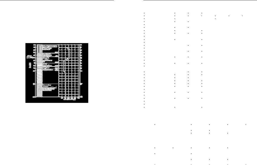
The researching work and design of the reinforced embankment was carried out byengineers ofAlberta University.Testingembankment is 12 mof high,inclinationof 1:1. Embankment consists of four sections, three of them reinforced by different type of geogrid and fourth section non reinforced, see Figure 1.

Figure 1. Tested embankment

ThefoundationsoilwasstudiedbyHofmann(1989). Fourboreholesweredrilled at the test fill site using a wet rotary drill rig which allowed Shelby tube samples, 73

289

Численные методы расчетов в практической геотехнике

mm in diameter by 610 mm long, to be taken (B.A. Hofmann). The shelby tubes were taken byHofmann about depth of 10 min borehole 1, 3 and 4. In borehole 2, however,

drilling was continued down to clay shale bedrock at 27 m, without sampling. Examination of the material removed as drilling progressed showed that the

grey sand was continuous to the bedrock. Alberta Transportation and Utilities drilled and logger a total of 70 boreholes at various locations along the new alignment of Highway 60 to the depth at 20 m. Atypical borehole profile is shown in Figure 2 and results of laboratory tests of the foundation and filling soils obtained by Hofmann and Alberta Transportation is shown in Table 1. The groundwater table is 5 m below the ground surface (Barbara, A. Hofman, 1989).

Figure 2. Profile of foundation soil

For the reinforcing of the test embankment it was chosen to use three types of hightensilestrengthgeogrids:TensarSR2,SignodeTNX5001 andParagrid50S.Their physical properties provided by the manufacturers are summarized in Table 2 (Y. Liu). Beforethegeogridswereused inthetestfill,load-extentionprorertiesofreinforcement materials were obtained from unconfined tests such as the grab tensile test, the steip tensile test and wide width tensile test.

Therewere defectsin theParagrid material supplied and placed inthe test fill. It was found during laboratory tests that some of the high strength fibers in the tension members were weakened or damaged at the intersections of the grids. This damage was most likely caused byoverheatingof the polypropylene sheathduring the welding process.DuringtestofSignodesectionitwasfoundthatmostinstrumentationdamaged and not good for interpretation of the instrumentations results, therefore it was chosen to use Tensar section for the FEM analysis by Plaxis (Y. Liu, 1992).

A.Zh. Zhussupbekov, R.E.Lukpanov, A.Tulebekova, I.O.Morev,Y.B.Utepov, D.Chan

Table 1

Properties of upper foundation soil and filling soil

Численные методы расчетов в практической геотехнике

3.2D SIMULATION OFREINFORCED EMBANKMENTBYPLAXIS

Properconstructivmodelsof the testfilland material parametersshould be used inthefiniteelementanalysis.Nonlinearstress-strainrelationshipwereusedformodeling the behavior of the soil, and the model parameters were derived based on labaratory test results. The load-strain behavoiur of geosynthetic under test conditions of 200C and rate 2% per minute were used to model the reinforcement (Chang-Tok Yi, 1995).

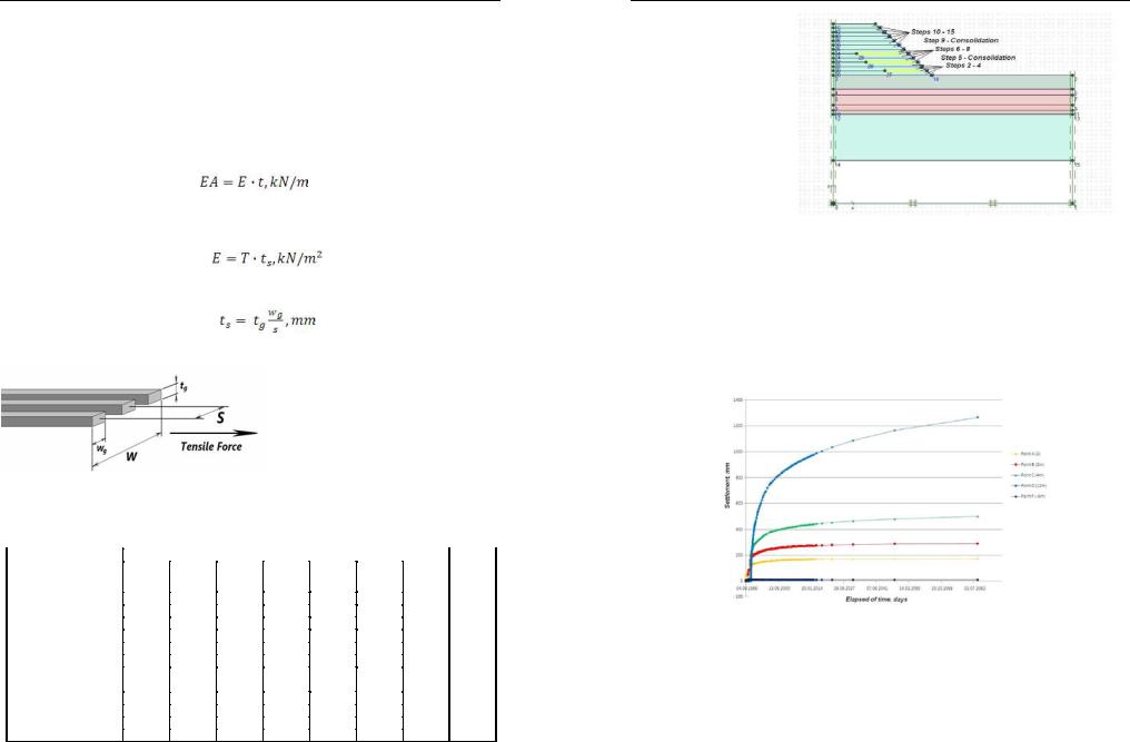
For analysis of reinforced embankment by Plaxis we need to know only one perameterofgeogridisanelasticnormal(axial)stiffenessofgrids,whichcanbedefined:

(1)

where EA is elastic normal (axial) stiffeness of grids, kN/m; E is Young‘s modulus of the geotextile, kN/m2; t is thickness of the fabric, m.

Young‘s modulus of the geotextile is obtained from having tensile force:

(2)

where T is tensile force, kN/m; ts is trasformed thickness of geogrid, mm. Transformed thickness of the gegrid defined by next equation:

Magnitude of normal stiffness of Tensar SR2, EA= 51kN/m.

A.Zh. Zhussupbekov, R.E.Lukpanov, A.Tulebekova, I.O.Morev,Y.B.Utepov, D.Chan

It was chosen several interested us points for the analysis of embankment settlement. Taken points are corresponds to positions of instrumentations.

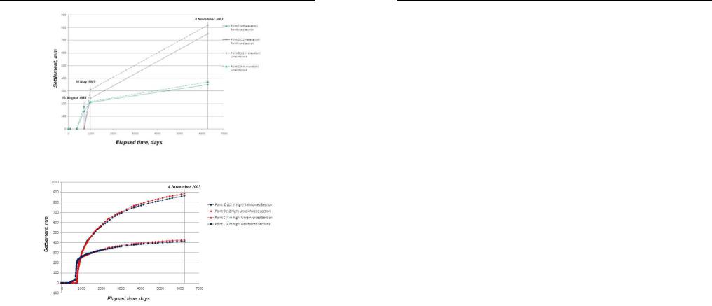
According results full settlement due to of full consolidation will be in 2602 year, but forpoint D (12 m) the settlement will be neglected small at 2055, with rate of 0.5 mm per year. For pointA(0 m) same rate of settlement occur after 2001, for point B (2m) – 2012, point C (4 m) – 2025, point F (-6 m) after two years. Predictable settlement curve is shown on Figure 5.

Figure 5. Predictable settlement curve

The settlement of unreinforced section almost has the same value as reinforced section.As in-situ test results shown the magnitude of point D settlement (12 m high) is 820 mm for unreinforced section whereas reinforced section settlement is 750 mm. For the curiously Plaxis results has the same picture. Unreinforced and reinforced section settlements obtained by in-situ observation and Plaxis simulations are shown on Figure 6 and 7 (Chan, D., Lukpanov, R., 2008).

Численные методы расчетов в практической геотехнике

Figure 6. Unreinforced and reinforced section settlements difference by in-situ

Figure 7. Unreinforced and reinforced section settlements difference by Plaxis

Youcanseethatsettlementofreinforced sectionslightlyhigherthanunreinforced section settlement. This may also raise the doubt that there are no effects of reinforced application, but real observation can help us to understand the mechanism of stability and failure. Redistribution load among construction parts and transmission the stress from the overloading zone to the adjacent underloading zone, lead to smoothly deformation of reinforced section and failure effects of unreinforced section.

4.CONCLUSIONS

By obtained results of settlements we can conclude that reinforcement of earth embankment play a very big role for the embankment stability for a long time. As results of Plaxis simulation of soft clay embankment showed that settlement of the

294

В.М. Улицкий, А.Г. Шашкин

high point (12 m) conventionally stops at 2055 and predictable magnitude of full settlement is 1150 mm. Following settlement is neglected small with rate 0.5 mm per year.Thesettlementsvaluevariousfrom914to920mmat2008 andstillcontinuewith rate 9–10 mm per year.

Insignificant settlement difference of reinforced and unreinforced section can mislead us of application necessity of reinforcement. Fromthe aforesaid we can make wrong conclusion that there is no effect of reinforcement, but real embankment observationcorroboratedreinforcedmodelaslongasunreinforcedsectionhadafailure effects of the shallow slope, whereas reinforced section smoothly deformed without any rapture, collapse or crumble effects.

In fine fulfilled researching work approved reinforcement model as one of the effective earth improvement technology concrete.

References

1.Barbara,A. Hofman, Evaluation of the soil properties of the Devon test fill. A thesis submittedto thefacultyof graduatestudies andresearchin partial fulfillment of therequirements for the degree of masters of science. Department of civil engineering. Edmonton,Alberta. 1989;

2.LiuYixin,Performanceofgeogridreinforcedclayslopes.AthesissubmittedtotheFaculty of Graduate Studies and Research in partial fulfillment of the requirements for the degree of Doctor of Philosophy. Department of civil engineering. Edmonton,Alberta. 1992;

3.Chang-TokYi. InterfaceModelingofGeosynthetic Reinforcement,1995, Libraryof UA;

4.Chan, D., Lukpanov, R. «Influence of Reinforcement to Horizontal and Vertical Displacement Development». International Scientific Practical Conference dedicated to the 45th

Anniversary of the TCEI,Astana, 2009.

ВПОРЯДКЕ ДИСКУССИИ

УДК 624.13

В.М. Улицкий (ПГУПС, Санкт-Петербург), А.Г. Шашкин (Проектный институт «Геореконструкция», Санкт-Петербург)

НАУЧНО-ТЕХНИЧЕСКОЕОБОСНОВАНИЕУСТРОЙСТВА ПОДЗЕМНОГООБЪЕМАВТОРОЙСЦЕНЫМАРИИНСКОГОТЕАТРА

ВУСЛОВИЯХСЛАБЫХ ГЛИНИСТЫХГРУНТОВ

Встатье приводится сравнение двух концепций устройства подземного объема здания новой сцены Мариинского театра. Первая концепция, предполагающая превентивное устройство жесткой коробчатой конструкции по контуру котлована, удерживающей массив грунта от горизонтальных смещений, была проверена на опытном котловане и обеспечивала сохранность прилегаю-

295

Численные методы расчетов в практической геотехнике

щейзастройки,ноне былареализованана практике.Техническиерешения,описываемыеавторами,основаныначисленноммоделировании,развивающемидеи проф.А.Б.Фадеева.Напрактикебылаосуществлена другаяконцепция,предусматривающая реализацию метода top-down всего с одним распорным уровнем, обладающаясущественно болеевысокой податливостью.

Новому зданию Мариинского театра, которое возводится рядом с исторической сценой прославленного театра, уделялось немало внимания в средствах массовой информации и в специальных изданиях. Все началось с проведения первого в России международного архитектурного конкурса (таких конкурсов не проводилось с 1930-х гг.), на котором победил проект знаменитого французского архитектора Доминика Перро.

Перро представил театр как рационально функционирующий комплекс разновысоких объемов зрительного зала, сцены, арьерсцены, репетиционных залов, служебных итехнических помещений, перекрытый оболочкой полупрозрачного «золотого кокона». Не будем судить, насколько гармонично вписалось бы это здание в архитектурную ткань Санкт-Петербурга, отметим лишь, что оно никогонеоставилобыравнодушнымисталобы объектомповышенного интереса жителей и гостей города. То, что реализуется на этом месте сегодня, не способно вызвать каких-либо сильных эмоций. Это – продукт смены трех проектировщиковичетырехзаказчиковданногообъекта.Сегодняещерано давать окончательную эстетическую оценку данному явлению, но итоги строительства подземного объема здания подвести уже можно.

Под всем зданием театра Д.Перро предусматривалось устройство трехэтажногоподземного объемасотметкойпола нижнего этажа–10,2 мБС.Отметка покрытия самого верхнего этажа +42,6 м. Размеры здания в плане 154×77 м (неправильная трапеция).

Весь надземный объем здания был разделен деформационными и звуко- изоляционными(акустическими)швамина11независимыхдеформационно-аку- стических блоков.

Исключение составлял нижний подземный этаж (ниже относительной отметки – 8,0) о котором следует сказать особо. Поскольку в нем не предполагалось функционирование каких-либо театральных технологий и габариты помещений не были строго лимитированы, специалисты института «Геореконструкция» предложили превратить пространство этого этажа в жесткую коробчатую конструкцию с поперечными и продольными балками-стенками. Такой конструктивныйприемпозволилнамрешитьсразунесколько задач:1)создатьединую жесткую коробчатую платформу под всем зданием, позволяющую более равномернораспределитьнагрузкинасвайноеоснование;2)исключитьпроблемупро- давливаниясваямисвайногоростверкапутемразмещениясвайподбалками-стен- ками; 3) благодаря коробчатой конструкции стал возможен весьма рациональный вариант устройства подземного объема здания (подробнее об этом будет сказано ниже).

296

В.М. Улицкий, А.Г. Шашкин

Отметки дневнойповерхности территории, на которой строился театр, варьируютот+2,3до+2,5, что соответствуетнаиболеенизкимотметкамлиториновой террасы. Территория находится в дельте р.Нева. С четырех сторон к проектируемому зданию примыкают: Крюков канал (расстояние 15м), Минский пер. (расстояниедо ближайшейзастройки~15м),пр.Декабристовиул. СоюзаПечатников (расстояние до ближайшей застройки ~30м).

Под насыпными грунтами она образована послеледниковыми, позднеледниковымииледниковымиотложениями. Техногенные отложенияtg IV иозерноморские отложения ml IV – пески пылеватые и мелкие распространены до абс. отм. – 2,6…-3,3 м БС; озерно-ледниковые отложения lgIII – суглинки мягко-

итекучепластичные - до абс. отм. – 10,8…-12,6 м БС; ледниковые gIII cуглинки мягко- и тугопластичные, супеси пластичные до абс. отм. – 21,3…-24 м БС; толщучетвертичныхотложенийподстилаютпротерозойскиеглиныV2кt2 тугопластичные и полутвердые.

Вданной геотехнической ситуации наиболее эффективным является вариант свайных фундаментов, опирающихся на слабосжимаемые протерозойские отложения. Глубина погружения свай от дневной поверхности составляет около 29м. Посколькунагрузки от зданияпередаютсянаслоипротерозойских отложений, кровля которых находится на 14–15м ниже дна котлована, нет оснований ожидать расструктуривания этих грунтов, а также существенной релаксации напряжений при разгрузке массива в процессе разработки котлована. В этом случае можно вполне обоснованно учитывать эффект разгрузки основания при выемке грунта, что согласуется стребованием отечественных норм.Приучете веса вынутого грунта дополнительные нагрузки на основание оказываются незначительными, что позволяет считать вариант свайных фундаментов близким к безосадочному.

При устройстве подземного объема необходимо обеспечить безопасность окружающей застройки, а для этого необходимо решить две основные проблемы: обеспечение минимальных горизонтальных смещений ограждения котлована и исключение водопритока в котлован.

Очевидно, что при откопке котлована ниже уровня грунтовых вод необходимо водопонижение. Возникновение депрессионной воронки вокруг котлована может сопровождаться выносом частиц грунта из-под фундаментов соседних зданий или сохраняемых конструкцийи увеличением эффективных напряжений в грунте. Оба явления могут привести к росту осадок окружающих зданий. В рассматриваемом проекте следовало тщательно проработать вопрос устройства противофильтрационной завесы (ПФЗ). Очевидно, что ПФЗ должна быть заведенавнадежныйводоупор,вкачествекоторогомогутрассматриватьсяполутвердые моренные отложения. Наличие на сравнительно небольших глубинах (около 23 м БС) твердых глин венда (протерозоя) позволяет рассматривать их

ив качестве надежного опорного слоя и гарантированного водоупора. В рамках

настоящейконцепцииглубинапогружениянаружногоограждениякотлованабыла принята равной 22–24 м (до слоя протерозойских отложений).

297