Longitudinal approximations reduced order models

THE LONG PERIOD MODE APPROXIMATION

The long period mode or phugoid mode is possible to characterize as a gradual interchange of potential and kinematic energy about equilibrium altitude and airspeed. This is illustrated in Fig.5 (a). Here we see that the long period mode is characterized by changes in pitch attitude, altitude and velocity at a nearly constant angle of attack. An approximation to the long –period mode can be obtained by neglecting the pitch moment equation and assuming that the change in angle of attack is zero, i.e.

.

Making these assumptions, the homogeneous longitudinal state equations reduce to the following:

.

The eigenvalues of the long period are obtained by solving the equation

or .

Expanding the above determinant yields

or .

The frequency and damping ratio can be expressed as

, .

If we neglect the compressibility effects, the frequency and damping ratios for the long period motion can be approximated by the following equations:

, , where is a lift to drag ratio.

To improve damping of the phugoid motion, the designer would have to reduce lift to drag ratio of the airplane.

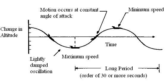
a - Phugoid Mode

b - Short – period Mode

Figure 5 Sketch of the phugoid and short – period motions

THE SHORT PERIOD MODE APPROXIMATION

It has already been established that the short period pitching oscillation is almost exclusively an oscillation in which the principal variables are pitch rate q and incidence α, the speed remaining essentially constant, thus u=0. Therefore, the speed equation and the speed dependent terms may be removed from the longitudinal equations of motion given in general form below

(8)

since they are all approximately zero in short term motion, the revised equations may be written in the following way:

(9)

By assuming that the equations of motion are referred to aircraft wind axes and that the aircraft is initially in steady level flight then θ_e ≡ α_e = 0 and U_e=V₀, it follows that z_θ = m_θ = 0. Equation (9) then reduces to its simplest possible form:

or

.

The above equation can be written in terms of angle of attack by using the relationship

.

In addition, one can replace the derivatives due to and with derivatives due to and by using following equations. The definition of the derivative is

.

In a similar way it is possible to show that

, .

Using the above expressions, the state equations for short – period approximation can be rewritten as

.

The eigenvalues of the state equation can be determined by solving the equation

which yields .

The characteristic equation for above determinant is

,

or in term of damping ratio and frequency

, .

Standard task for laboratory work 5

The equation of motion referred to body axis system, arranged in state space form is given with quadruple of matrices A, B, C, D. It is necessary:

• obtain the reduced order model for short period and phugoid modes;

• evaluate by hand the transfer function describing pitch attitude response to elevator deflection for short period mode;

• find the longitudinal eigenvalues and eigenvectors and compare with the results obtained by using short period and phugoid modes, respectively;

• determine the period of the short period and phugoid modes;

• write down the longitudinal characteristic equation and state whether the airplane is stable or not.