

Laboratory work № 7 analog filtert design brief theoretical information
A filter is one, which rejects unwanted frequencies from the input signal and allows the desired frequencies to obtain the required shape of output signal.
The range of frequencies of signal that are passed through the filter is called passband and those frequencies that are blocked is called stopband.
The filters are of different types:
1. Low-pass filter (LPF). 2. High-pass filter (HPF).
3. Band-pass filter (BPF). 4. Band-stop (reject) filter (BSF).
An ideal
filter will have an amplitude response that is unity (or at a fixed
gain) for the frequencies of interest (called the pass
band)
and zero everywhere else (called the stop-band).
The frequency at which the response changes from pass-band to
stop-band is referred to as the cut-off
frequency,
![]() .
Figure 1(a) shows an idealized low-pass filter. In this filter the
low frequencies are in the pass band and the higher frequencies are
in the stop band. The PHF passes the high frequencies (they are in
the pass band) and all the low frequencies are in the stop band
(Figure 1 b – idealized HPF). If a high filter and low –pass
filter are cascaded, a
band pass
filter is created. The BPF passes a band of frequencies berween a
lower cut-off frequency,
.
Figure 1(a) shows an idealized low-pass filter. In this filter the
low frequencies are in the pass band and the higher frequencies are
in the stop band. The PHF passes the high frequencies (they are in
the pass band) and all the low frequencies are in the stop band
(Figure 1 b – idealized HPF). If a high filter and low –pass
filter are cascaded, a
band pass
filter is created. The BPF passes a band of frequencies berween a
lower cut-off frequency,
![]() and an upper frequency,
and an upper frequency,
![]() .
The frequncies below
and above
are in the stop band. An idealized BPF is shown in Figure 1(c). The
band-stop
filter passes frequencies below
and above
.
The band from
to
are in the stop band. Figure 1 (d) shows an idealized BSF.
.
The frequncies below
and above
are in the stop band. An idealized BPF is shown in Figure 1(c). The
band-stop
filter passes frequencies below
and above
.
The band from
to
are in the stop band. Figure 1 (d) shows an idealized BSF.
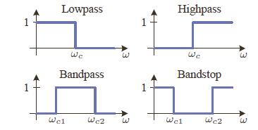
Figure 1 Idealized Filter Frequency Responses
The idealized filters defined above, unfortunately, cannot be easily built. The transition from pass band to stop band will not be instantaneous, but instead there will be a transition region. Stop band attenuation will not be infinite. Practical filters are usually designed to meet a set of specifications.
To obtain a physically realizable filter, it is necessary to relax some of the requirements of the ideal filters. Figure 2 shows the frequency characteristics of physically realizable versions of various ideal filters. The upper and lower bounds for the gains are indicated by the shaded line, while examples of the frequency characteristics of physically realizable filters that satisfy the specified bounds are shown using bold lines. These filters are referred to as non-ideal or practical filters and are different from the ideal filters in the following two ways:
The gains of the practical filters within the pass and stop bands are not constant but vary within the following limits:
pass
bands ![]() ;
;
stop
bands ![]() .
.
The
oscillations within the pass and stop bands are referred to as
ripples. In Figure 2, the pass band ripples are constrained to a
value of
![]() for LPF, HPF, and BPF. In the case of BSF, the pass band ripples are
limited to
for LPF, HPF, and BPF. In the case of BSF, the pass band ripples are
limited to
![]() and
and
![]() ,
corresponding to the two pass band. Similarly, the stop band ripples
in Figure 2 are constrained to
,
corresponding to the two pass band. Similarly, the stop band ripples
in Figure 2 are constrained to
![]() for LPF, HPF and BSF. In the case of BSF, the stop band ripples are
limited to
for LPF, HPF and BSF. In the case of BSF, the stop band ripples are
limited to
![]() and
and
![]() for the two stop bands of the BSF.
for the two stop bands of the BSF.
Transition bands of non-zero bandwidth are included in between the pass and stop bands of the practical filters. Consequently, the discontinuity at the cut-off frequency of the ideal filters is eliminated.
CUT-OFF FREQUENCY
An important parameter in the design of continuous time filters is the cut-off frequency of the filter, which is defined as the frequency at which the gain of the filter drops to 0.7071 times its maximum value. Assuming a gain of unity within the pass band, the gain at the cut-off frequency is given by 0.7071 or -3 dB on a logarithmic scale. Since the cut-off frequency lies typically within the transitional band of the filter, for a low pass filter
![]() .
.
Since the
equality
![]() implies a transitional band of zero bandwidth, this equality is only
valid for ideal filters.
implies a transitional band of zero bandwidth, this equality is only
valid for ideal filters.
Lowpass and highpass filters usually have the following requirements:
Passband range;
- Stopband range;
Maximum ripple in the passband;
Minimum attenuation in the stopband.
There are four popular types of standard filters:
- Butterworth
- Chebysev Type I
- Chebyshev Type II
- Elliptic.
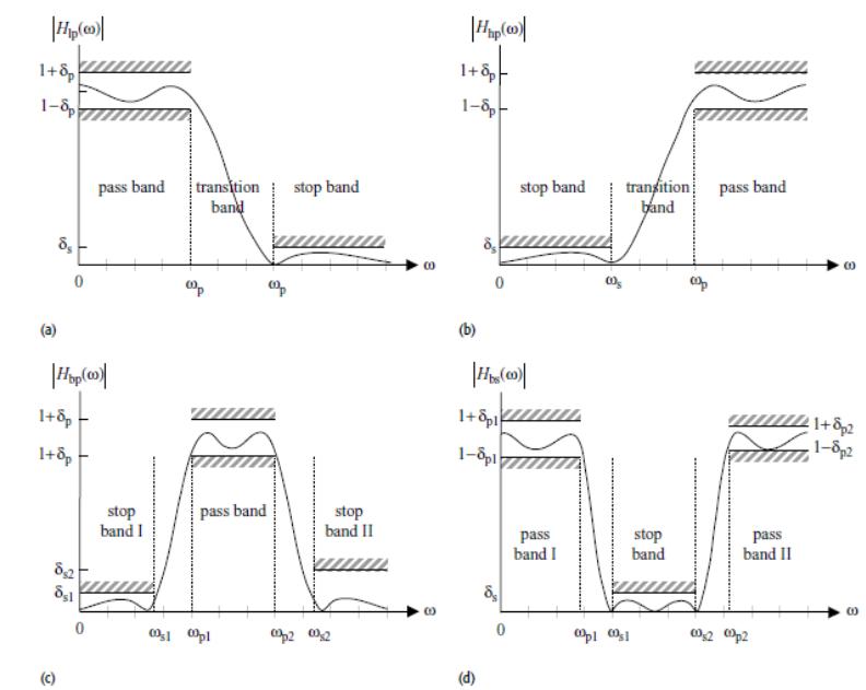
Figure 2 Frequency Characteristics of Practical Filters
(a) Practical Low Pass Filter; (b) Practical High Pass Filter; (c) Practical Band Pass Filter; (d) Practical Band Stop Filter
NORMALIZED TRANSFER FUNCTIONS
A normalized low pass transfer function is one in which the pass band edge radian frequency is set to 1 rad/sec. Of course, this seems a rather unusual frequency, since seldom would a low pass filter be required to have such a low frequency. However, the technique actually allows the filter designer considerable latitude in designing filters because a normalized transfer function can easily be unnormalized to any other frequency.
BUTTERWORTH FILTERS
The Butterworth filter is the best compromise between attenuation and phase response. It has no ripple in the pass band or the stop band, and because of this is sometimes called maximally flat filters. The Butterworth filter achieves its flatness at the expense of a relatively wide transition region from pass band to stop band, with average transient characteristics. The low pass Butterworth polynomial has an all-pole transfer function with no finite zeros present.
The normalized Butterworth low pass filter of the n-th order is given by magnitude response function
![]() ,
,
where n is the order of the filter, n=1, 2,…
The normalized poles of the Butterworth filter fall on the unit circle (in the s-plane). The pole positions in left-half plane are defined via following relation
![]() , (1)
, (1)
where
![]() ;
k=1,
2,…, n.
(2)
;
k=1,
2,…, n.
(2)
Draw your attention, that the poles positions in the right-half plane are defined as follows
![]() ,
,
where
![]() are defined by equation (2); k=1,
2,…, n.
k
is the pole pair number; and n
is the number of poles.
are defined by equation (2); k=1,
2,…, n.
k
is the pole pair number; and n
is the number of poles.