

LABORATORY WORK № 5
AIRCRAFT RESPONSE TRANSFER FUNCTIONS
AIRCRAFT STABILITY AND DYNAMICS
BRIEF THEORETICAL REVIEW
Dynamic stability is a very important field for the understanding of aircraft flying and handling qualities.
While static stability determines the steady state, or trim, of an aircraft, the dynamic stability is related to the dynamic, or transient, part of the aircraft response to pilot or disturbance inputs. Therefore, although the steady state is the ultimate objective of a pilot, the way an aircraft behaves to reach that end, i.e. the transient response, may be more determinative for pilots when assessing a certain configuration for accomplishing a specified task. Since dynamic stability defines the transient response of a system its characteristics are not dependent on just a few basic aerodynamic parameters, but on the more complex relationships and interaction of all characteristics. The equations of motion represent the complete analytical source of an aircraft response, both transient and steady state, to pilot inputs. However, the analysis of the complete non-linear equations of motion is very complex. Thus, the usual approach is to assume small perturbations and to linearize the equations of motion around a flight condition, to obtain the well-known state space model. A further simplification is to separate the longitudinal motion from the lateral – directional motion due to the symmetry of the airplane.
The possibility of separating the longitudinal and lateral- directional stability aircraft motion makes it easier to analyze and understand the aircraft behaviour.
AIRCRAFT RESPONSE TRANSFER FUNCTIONS
Aircraft response transfer functions describe the dynamic relationships between the input and output variables. The relationships are indicated diagrammatically in Fig.1 and clearly, a number of possible input–output relationships exist. When the mathematical model of the aircraft comprises the decoupled small perturbation equations of motion, transfer functions relating longitudinal input variables to lateral output variables do not exist and vice versa. This may not necessarily be the case when the aircraft is described by a fully coupled set of small perturbation equations of motion. For example, such a description is quite usual when modelling the helicopter. All transfer functions are written as a ratio of two polynomials in the Laplace operator s. All proper transfer functions have a numerator polynomial which is at least one order less than the denominator polynomial although, occasionally, improper transfer functions crop up in aircraft applications. For example, the transfer function describing acceleration response to an input variable is improper, the numerator and denominator polynomials are of the same order. Care is needed when working with improper transfer functions as sometimes the computational tools are unable to deal with them correctly. Clearly, this is a situation where some understanding of the physical meaning of the transfer function can be of considerable advantage.
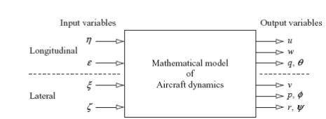
Figure 1 Aircraft input – output relationships
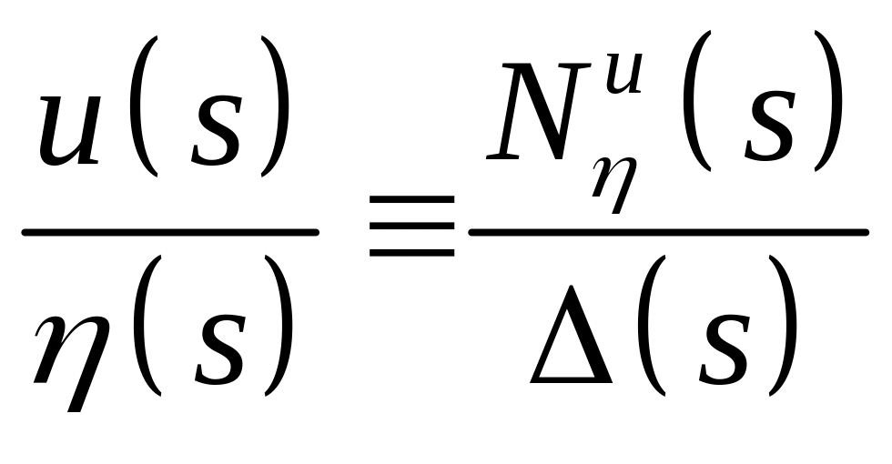
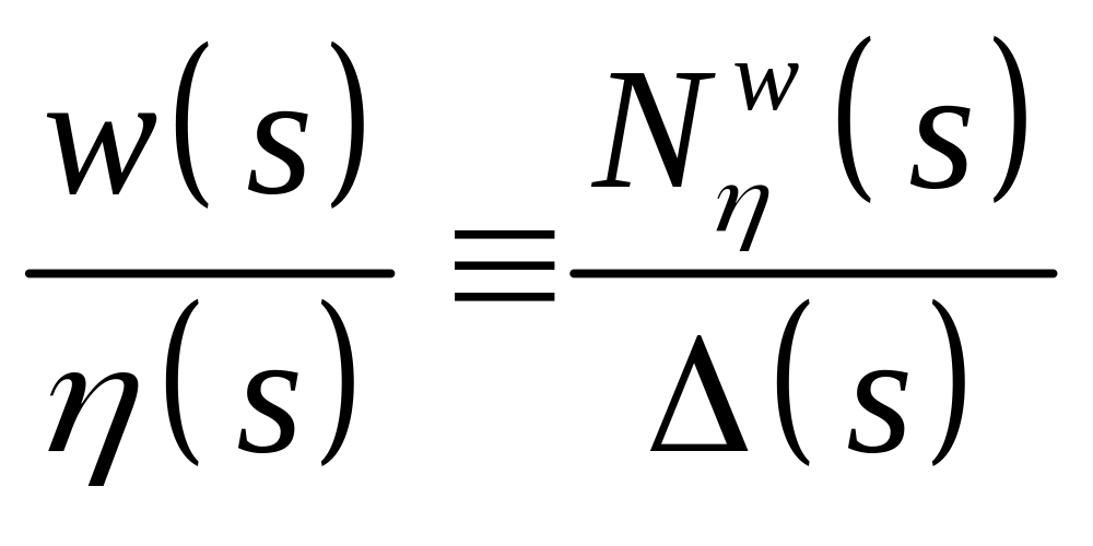
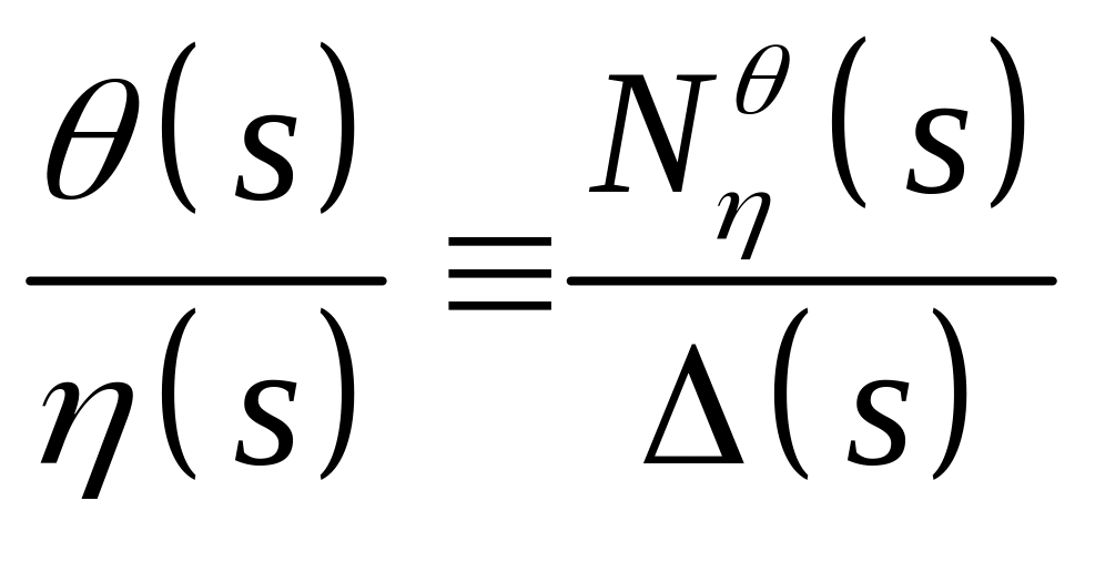
A shorthand notation is used to represent aircraft response transfer functions. For example, pitch attitude θ(s) response to elevator η(s) is denoted:
![]() ,
,
where
![]() is the unique numerator polynomial in s
relating
pitch attitude response to elevator input and
is the unique numerator polynomial in s
relating
pitch attitude response to elevator input and
![]() is the denominator polynomial in s
which
is common to all of the longitudinal response transfer functions.
is the denominator polynomial in s
which
is common to all of the longitudinal response transfer functions.
The denominator polynomial Δ(s) is called the characteristic polynomial and when equated to zero defines the characteristic equation. Thus, Δ(s) completely describes the longitudinal or lateral stability characteristics of the aeroplane as appropriate and the roots, or poles, of Δ(s) describe the stability modes of the aeroplane. Thus, the stability characteristics of an aeroplane can be determined simply on inspection of the response transfer functions.
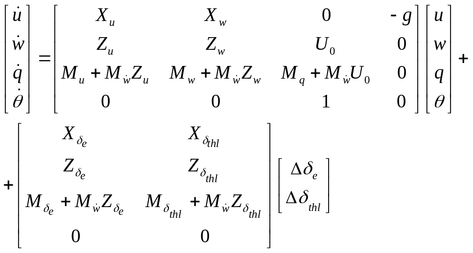
Longitudinal equations of motion
Decoupled longitudinal motion is motion in response to a disturbance which is constrained to the longitudinal plane of symmetry, the oxz plane, only. The motion is therefore described by the axial force X, normal force Z, and the pitching moment M equations only. Since no lateral motion is involved the lateral motion variables v, p and r and their derivatives are all zero. Also, decoupled longitudinal – lateral motion means that the aerodynamic coupling derivatives are negligibly small and may be taken as zero.
Thus, the equation of longitudinal motion referred to the body axes, taking into account zero initial conditions and since small perturbation only is considered possible to write:
![]()
![]()
![]()
(1)
Equations
(1) are the most general form of the dimensional decoupled equations
of longitudinal symmetric motion referred to aeroplane body axes. In
(1) the dimensional variables are denoted by
![]() .
.
If it is assumed that the aeroplane is in level flight and the reference axes are wind or stability axes then
![]()
![]() and
and
![]() ,
and
,
and
![]()
And the equations simplify further to
![]()
![]()
(2)
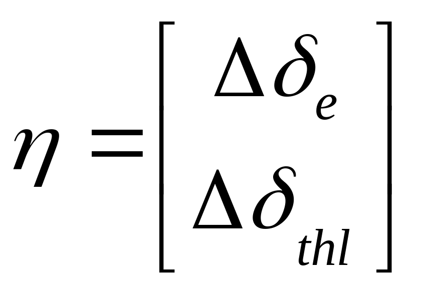
Variables
![]() ,
,
![]() in
equation (2) stand for elevator and throttle deflection,
respectively. Since the longitudinal motion of aeroplane is described
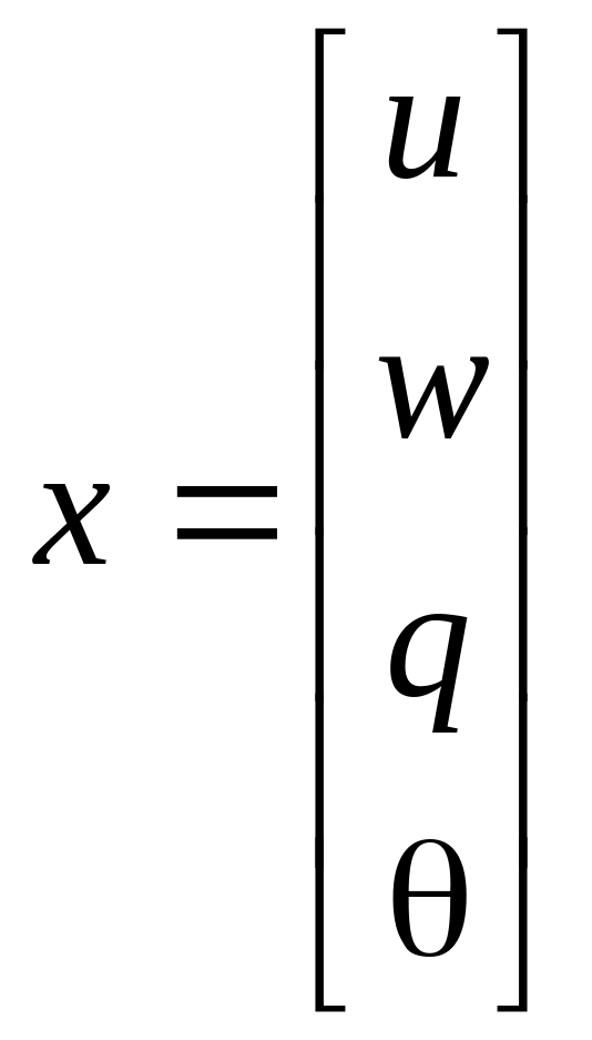
by four state variables
in
equation (2) stand for elevator and throttle deflection,
respectively. Since the longitudinal motion of aeroplane is described
by four state variables
![]() and
and
![]() and four differential equations are required. Thus the additional
equation is the auxiliary equation relating pitch rate to attitude
rate, which small perturbation is
and four differential equations are required. Thus the additional
equation is the auxiliary equation relating pitch rate to attitude
rate, which small perturbation is
![]() .
.
STATE VARIABLE REPRESENTATION OF THE EQUATIONS OF MOTION
The motion, or state, of any linear dynamic system may be described by a minimum set of variables called the state variables. The number of state variables required to completely describe the motion of the system is dependent on the number of degrees of freedom the system has. Thus the motion of the system is described in a multidimensional vector space called the state space, thee number of state variables being equal to the number of dimensions. The equation of motion, or state equation, of the linear time invariant (LTI) multi-variable system is written:
![]() ,
,
where x(t) is the column vector of n state variables called the state vector;
u(t) is the column vector of m input variables called the input vector.
A is the (nxn) state matrix;
B is the (nxm) input matrix;
y(t) is the column vector of r output variables called the output vector.
C is the (r xn) output matrix.
D is the (rxm) direct matrix.
Hence, in terms of dimensionless derivatives the equations of longitudinal motion in the state space form is written as follows:
 ,
,
where the
state space vector x
and
control vector
![]() are given by
are given by
The longitudinal response transfer functions
The Laplace
transform of the differential quantities
![]() and
and
![]() ,
for example, are given by
,
for example, are given by
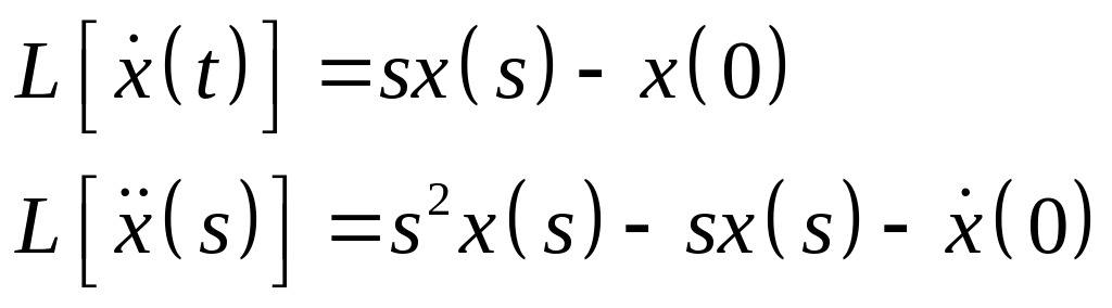 ,
,
where
![]() and
and
![]() are initial values of
are initial values of
![]() and
respectively at t=0.
Now, taking Laplace transform of the longitudinal equations of motion
(1) , reffered to body axes, assuming zero initial conditions and
since small perturbation motion only is considered write
and
respectively at t=0.
Now, taking Laplace transform of the longitudinal equations of motion
(1) , reffered to body axes, assuming zero initial conditions and
since small perturbation motion only is considered write
![]() ,
,

![]()
![]() (3)
(3)
Let us rewrite equation (3) in matrix format
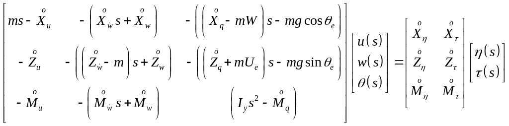 . (4)
. (4)
Cramer’s
rule can now be applied to obtain the longitudinal response transfer
functions, for example, to obtain the transfer functions describing
response to elevator. Assume, therefore, that the thrust remains
constant. This means that the throttle is fixed at its trim setting
![]() and
and
![]() .
Therefore, after dividing through by
.
Therefore, after dividing through by
![]() equation (4) may be simplified to
equation (4) may be simplified to
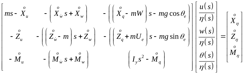 (5)
(5)
Cramer’s rule may be applied directly and the elevator response transfer functions are given by
 ,
,
 ,
,
 .
.
Since the
Laplace transform of equation (3) is
![]() the pitch rate response transfer function follows directly
the pitch rate response transfer function follows directly
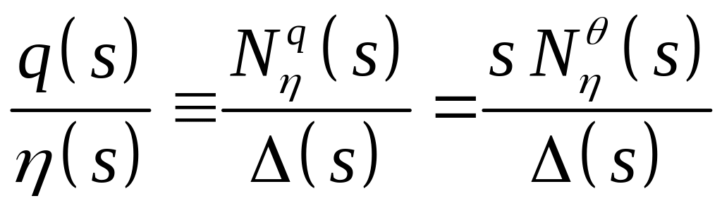 .
.
The
numerator polynomial for vertical component of true airspeed,
![]() is given as follows
is given as follows
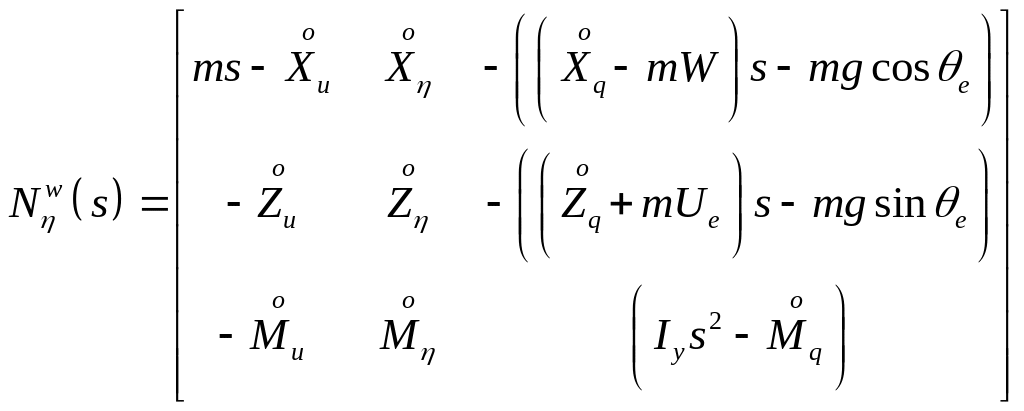 ,
,
And the common denominator for transfer functions takes the following form
 ,
,
Hence,
.
The thrust
response transfer functions may be derived by assuming the elevator
to be fixed at its trim value, thus
![]() ,
and
,
and
![]() is written in place of
.
Then the derivatives
is written in place of
.
Then the derivatives
![]() ,
,
![]() ,
,
![]() are
replaced by
are
replaced by
![]() ,
,
![]() ,
,
![]() .
.