

clustering
.pdf304 |
· |
A. Jain et al. |
strong assumptions (often multivariate Gaussian) about the multidimensional shape of clusters to be obtained. The ability of new clustering procedures to handle concepts and semantics in classification (in addition to numerical measurements) will be important for certain applications [Michalski and Stepp 1983; Murty and Jain 1995].
6.2Object and Character Recognition
6.2.1Object Recognition. The use of clustering to group views of 3D objects for the purposes of object recognition in range data was described in Dorai and Jain [1995]. The term view refers to a range image of an unoccluded object obtained from any arbitrary viewpoint. The system under consideration employed a viewpoint dependent (or viewcentered) approach to the object recognition problem; each object to be recognized was represented in terms of a library of range images of that object.
There are many possible views of a 3D object and one goal of that work was to avoid matching an unknown input view against each image of each object. A common theme in the object recognition literature is indexing, wherein the unknown view is used to select a subset of views of a subset of the objects in the database for further comparison, and rejects all other views of objects. One of the approaches to indexing employs the notion of view classes; a view class is the set of qualitatively similar views of an object. In that work, the view classes were identified by clustering; the rest of this subsection outlines the technique.
Object views were grouped into classes based on the similarity of shape spectral features. Each input image of an object viewed in isolation yields a feature vector which characterizes that view. The feature vector contains the first ten central moments of a normal-
ized shape spectral distribution, # ~h!,
H
of an object view. The shape spectrum of an object view is obtained from its range data by constructing a histogram of
shape index values (which are related to surface curvature values) and accumulating all the object pixels that fall into each bin. By normalizing the spectrum with respect to the total object area, the scale (size) differences that may exist between different objects are removed.
The first moment m1 is computed as the
weighted mean of # ~ !
H h :
# |
(1) |
m1 5 O~h!H~h!. |
h
The other central moments, mp, 2 # p
# 10 are defined as:
p # |
(2) |
mp 5 O~h 2 m1! H~h!. |
h
Then, the feature vector is denoted as
R 5 ~m1, m2, ´ ´ ´, m10!, with the range of each of these moments being
@21,1#.
Let 2 5 $O1, O2, ´ ´ ´, On% be a collection of n 3D objects whose views are present in the model database, }D. The ith view of the jth object, Oij in the database is represented by ^Lij, Rij&,
where Lij is the object label and Rij is the feature vector. Given a set of object
representations 5i 5 $^Li1, Ri1&, ´ ´ ´, ^Lim, Rim&% that describes m views of the ith object, the goal is to derive a partition of the views, 3i 5 $Ci1, Ci2, ´ ´ ´, Ciki%. Each cluster in 3i con-
tains those views of the ith object that have been adjudged similar based on the dissimilarity between the corresponding moment features of the shape spectra of the views. The measure of
dissimilarity, between Rij and Rik, is defined as:
$~Rij, Rik! 5 O10 ~Rijl 2 Rikl!2. (3)
l51
6.2.2 Clustering Views. A database containing 3,200 range images of 10 different sculpted objects with 320 views per object is used [Dorai and Jain 1995].
ACM Computing Surveys, Vol. 31, No. 3, September 1999
Data Clustering · 305
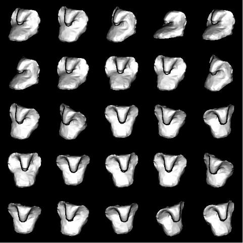
Figure 31. A subset of views of Cobra chosen from a set of 320 views.
The range images from 320 possible viewpoints (determined by the tessellation of the view-sphere using the icosahedron) of the objects were synthesized. Figure 31 shows a subset of the collection of views of Cobra used in the experiment.
The shape spectrum of each view is computed and then its feature vector is determined. The views of each object are clustered, based on the dissimilarity
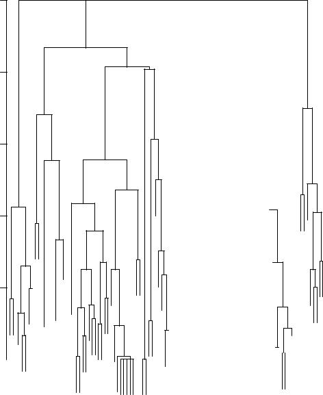
measure $ between their moment vectors using the complete-link hierarchical clustering scheme [Jain and Dubes 1988]. The hierarchical grouping obtained with 320 views of the Cobra ob-
ject is shown in Figure 32. The view grouping hierarchies of the other nine objects are similar to the dendrogram in Figure 32. This dendrogram is cut at a dissimilarity level of 0.1 or less to obtain compact and well-separated clusters. The clusterings obtained in this manner demonstrate that the views of each object fall into several distinguishable clusters. The centroid of each of these clusters was determined by computing the mean of the moment vectors of the views falling into the cluster.
Dorai and Jain [1995] demonstrated that this clustering-based view grouping procedure facilitates object matching
ACM Computing Surveys, Vol. 31, No. 3, September 1999

306 |
· |
A. Jain et al. |
|
|
|
|
|
|
|
|
|
|
|
|
|
|
|
|
|
|
|
|
|
|
|
|
|
|
|
|
|
|
|
|
||||||||||||||
|
0.25 |
|
|
|
|
|
|
|
|
|
|
|
|
|
|
|
|
|
|
|
|
|
|
|
|
|
|
|
|
|
|
|
|
|
|
|
|
|
|
|
|
|
|
|
|
|
|
|
|
|
|
|
|
|
|
|
|
|
|
|
|
|
|
|
|
|
|
|
|
|
|
|
|
|
|
|
|
|
|
|
|
|
|
|
|
|
|
|
|
|
|
|
|
|
|
|
|
|
|
|
|
|
|
|
|
|
|
|
|
|
|
|
|
|
|
|
|
|
|
|
|
|
|
|
|
|
|
|
|
|
|
|
|
|
|
|
|
|
|
|
|
|
|
|
||
|
0.20 |
|
|
|
|
|
|
|
|
|
|
|
|
|
|
|
|
|
|
|
|
|
|
|
|
|
|
|
|
|
|
|
|
|
|
|
|
|
|
|
|
|
|
|
|
|
|
|
|
|
|
|
|
|
|
|
|
|
|
|
|
|
|
|
|
|
|
|
|
|
|
|
|
|
|
|
|
|
|
|
|
|
|
|
|
|
|
|
|
|
|
|
|
|
|
|
|
|
0.15 |
|
|
|
|
|
|
|
|
|
|
|
|
|
|
|
|
|
|
|
|
|
|
|
|
|
|
|
|
|
|
|
|
|
|
|
|
|
|
|
|
|
|
|
|
|
|
|
|
|
|
|
|
|
|
|
|
|
|
|
|
|
|
|
|
|
|
|
|
|
|
|
|
|
|
|
|
|
|
|
|
|
|
|
|
|
|
|
|
|
|
|
|
|
|
|
|
|
0.10 |
|
|
|
|
|
|
|
|
|
|
|
|
|
|
|
|
|
|
|
|
|
|
|
|
|
|
|
|
|
|
|
|
|
|
|
|
|
|
|
|
|
|
|
|
|
|
|
|
|
|
|
|
|
|
|
|
|
|
|
|
|
|
|
|
|
|
|
|
|
|
|
|
|
|
|
|
|
|
|
|
|
|
|
|
|
|
|
|
|
|
|
|
|
|
||
|
|
|
|
|
|
|
|
|
|
|
|
|
|
|
|
|
|
|
|
|
|
|
|
|
|
|
|
|
|
|
|
|
|
|
|
|
|
|
|
|
|
|
|
|
|
|
|
|
|
0.05 |
|
|
|
|
|
|
|
|
|
|
|
|
|
|
|
|
|
|
|
|
|
|
|
|
|
|
|
|
|
|
|
|
|
|
|
|
|
|
|
|
|
|
|
|
|
|
|
|
|
|
|
|
|
|
|
|
|
|
|
|
|
|
|
|
|
|
|
|
|
|
|
|
|
|
|
|
|
|
|
|
|
|
|
|
|
|
|
|
|
|
|
|
|
|
|
|
|
|
|
|
|
|
|
|
|
|
|
|
|
|
|
|
|
|
|
|
|
|
|
|
|
|
|
|
|
|
|
|
|
|
|
|
|
|
|
|
|
|
|
|
|
|
|
|
|
|
|
|
|
|
|
|
|
|
|
|
|
|
|
|
|
|
|
|
|
|
|
|
|
|
|
|
|
|
|
|
|
|
|
|
|
|
|
|
|
|
|
|
|
|
|
|
|
|
|
|
|
|
|
|
|
|
|
|
|
|
|
|
|
|
|
|
|
|
|
|
|
|
|
|
|
|
|
|
|
|
|
|
|
|
|
|
|
|
|
|
|
|
|
|
|
|
|
|
|
|
|
|
|
|
|
|
|
|
|
|
|
|
|
|
|
|
|
|
|
|
|
|
|
|
|
|
|
|
|
|
|
|
|
|
|
|
|
|
|
|
|
|
|
|
|
|
|
0.0 |
|
|
|
|
|
|
|
|
|
|
|
|
|
|
|
|
|
|
|
|
|
|
|
|
|
|
|
|
|
|
|
|
|
|
|
|
|
|
|
|
|
|
|
|
|
|
|
|
|
|
|
|
|
|
|
|
|
|
|
|
|
|
|
|
|
|
|
|
|
|
|
|
|
|
|
|
|
|
|
|
|
|
|
|
|
|
|
|
|
|
|
|
|
|
|
|
|
|
|
|
|
|
|
|
|
|
|
|
|
|
|
|
|
|
|
|
|
|
|
|
|
|
|
|
|
|
|
|
|
|
|
|
|
|
|
|
|
|
|
|
|
|
|
|
|
|
|
|
|
|
|
|
|
|
|
|
|
|
|
|
|
|
|
|
|
|
|
|
|
|
|
|
|
|
|
|
|
|
|
|
|
|
|
|
|
|
|
|
|
|
|
|
|
|
Figure 32. Hierarchical grouping of 320 views of a cobra sculpture.
in terms of classification accuracy and the number of matches necessary for correct classification of test views. Object views are grouped into compact and homogeneous view clusters, thus demonstrating the power of the clusterbased scheme for view organization and efficient object matching.
6.2.3 Character Recognition. Clustering was employed in Connell and Jain [1998] to identify lexemes in handwritten text for the purposes of writerindependent handwriting recognition. The success of a handwriting recognition system is vitally dependent on its acceptance by potential users. Writerdependent systems provide a higher level of recognition accuracy than writ- er-independent systems, but require a large amount of training data. A writer-
independent system, on the other hand, must be able to recognize a wide variety of writing styles in order to satisfy an individual user. As the variability of the writing styles that must be captured by a system increases, it becomes more and more difficult to discriminate between different classes due to the amount of overlap in the feature space. One solution to this problem is to separate the data from these disparate writing styles for each class into different subclasses, known as lexemes. These lexemes represent portions of the data which are more easily separated from the data of classes other than that to which the lexeme belongs.
In this system, handwriting is cap-
tured by digitizing the ~x, y! position of the pen and the state of the pen point
ACM Computing Surveys, Vol. 31, No. 3, September 1999
(up or down) at a constant sampling rate. Following some resampling, normalization, and smoothing, each stroke of the pen is represented as a variablelength string of points. A metric based on elastic template matching and dynamic programming is defined to allow the distance between two strokes to be calculated.
Using the distances calculated in this manner, a proximity matrix is constructed for each class of digits (i.e., 0 through 9). Each matrix measures the intraclass distances for a particular digit class. Digits in a particular class are clustered in an attempt to find a small number of prototypes. Clustering is done using the CLUSTER program described above [Jain and Dubes 1988], in which the feature vector for a digit is
its N proximities to the digits of the same class. CLUSTER attempts to produce the best clustering for each value
of K over some range, where K is the number of clusters into which the data is to be partitioned. As expected, the mean squared error (MSE) decreases
monotonically as a function of K. The ªoptimalº value of K is chosen by identi-
fying a ªkneeº in the plot of MSE vs. K. When representing a cluster of digits by a single prototype, the best on-line recognition results were obtained by using the digit that is closest to that cluster's center. Using this scheme, a correct recognition rate of 99.33% was
obtained.
6.3 Information Retrieval
Information retrieval (IR) is concerned with automatic storage and retrieval of documents [Rasmussen 1992]. Many university libraries use IR systems to provide access to books, journals, and other documents. Libraries use the Library of Congress Classification (LCC) scheme for efficient storage and retrieval of books. The LCC scheme consists of classes labeled A to Z [LC Classification Outline 1990] which are used to characterize books belonging to dif-
Data Clustering · 307
ferent subjects. For example, label Q corresponds to books in the area of science, and the subclass QA is assigned to mathematics. Labels QA76 to QA76.8 are used for classifying books related to computers and other areas of computer science.
There are several problems associated with the classification of books using the LCC scheme. Some of these are listed below:
(1)When a user is searching for books in a library which deal with a topic of interest to him, the LCC number alone may not be able to retrieve all the relevant books. This is because the classification number assigned to the books or the subject categories that are typically entered in the database do not contain sufficient information regarding all the topics covered in a book. To illustrate this point, let us consider the book Algorithms for Clustering Data by Jain and Dubes [1988]. Its LCC number is `QA 278.J35'. In this LCC number, QA 278 corresponds to the topic `cluster analysis', J corresponds to the first author's name and 35 is the serial number assigned by the Library of Congress. The subject categories for this book provided by the publisher (which are typically entered in a database to facilitate search) are cluster analysis, data processing and algorithms. There is a chapter in this book [Jain and Dubes 1988] that deals with computer vision, image processing, and image segmentation. So a user looking for literature on computer vision and, in particular, image segmentation will not be able to access this book by searching the database with the help of either the LCC number or the subject categories provided in the database. The LCC number for computer vision books is TA 1632 [LC Classification 1990] which is very different from the number QA 278.J35 assigned to this book.
ACM Computing Surveys, Vol. 31, No. 3, September 1999
308 |
· |
A. Jain et al. |
(2)There is an inherent problem in assake of brevity in representation, the signing LCC numbers to books in a fourth-level nodes in the ACM CR clasrapidly developing area. For examsification tree are labeled using numerple, let us consider the area of neuals 1 to 9 and characters A to Z. For
ral networks. Initially, category `QP' in LCC scheme was used to label books and conference proceedings in this area. For example, Proceedings of the International Joint Conference on Neural Networks [IJCNN'91] was assigned the number `QP 363.3'. But most of the recent books on neural networks are given a number using the category label `QA'; Proceedings of the IJCNN'92 [IJCNN'92] is assigned the number `QA 76.87'. Multiple labels for books dealing with the same topic will force them to be placed on different stacks in a library. Hence, there is a need to update the classification labels from time to time in an emerging discipline.
(3)Assigning a number to a new book is a difficult problem. A book may deal with topics corresponding to two or more LCC numbers, and therefore, assigning a unique number to such a book is difficult.
Murty and Jain [1995] describe a knowledge-based clustering scheme to group representations of books, which are obtained using the ACM CR (Association for Computing Machinery Computing Reviews) classification tree [ACM CR Classifications 1994]. This tree is used by the authors contributing to various ACM publications to provide keywords in the form of ACM CR category labels. This tree consists of 11 nodes at the first level. These nodes are labeled A to K. Each node in this tree has a label that is a string of one or more symbols. These symbols are alphanumeric characters. For example, I515 is the label of a fourth-level node in the tree.
6.3.1 Pattern Representation. Each book is represented as a generalized list [Sangal 1991] of these strings using the ACM CR classification tree. For the
example, the children nodes of I.5.1 (models) are labeled I.5.1.1 to I.5.1.6. Here, I.5.1.1 corresponds to the node labeled deterministic, and I.5.1.6 stands for the node labeled structural. In a similar fashion, all the fourth-level nodes in the tree can be labeled as necessary. From now on, the dots in between successive symbols will be omitted to simplify the representation. For example, I.5.1.1 will be denoted as I511.
We illustrate this process of representation with the help of the book by Jain and Dubes [1988]. There are five chapters in this book. For simplicity of processing, we consider only the information in the chapter contents. There is a single entry in the table of contents for chapter 1, `Introduction,' and so we do not extract any keywords from this. Chapter 2, labeled `Data Representation,' has section titles that correspond to the labels of the nodes in the ACM CR classification tree [ACM CR Classifications 1994] which are given below:
(1a) I522 (feature evaluation and selection),
(2b) I532 (similarity measures), and
(3c) I515 (statistical).
Based on the above analysis, Chapter 2 of Jain and Dubes [1988] can be characterized by the weighted disjunction ((I522 I532 I515)(1,4)). The weights (1,4) denote that it is one of the four chapters which plays a role in the representation of the book. Based on the table of contents, we can use one or more of the strings I522, I532, and I515 to represent Chapter 2. In a similar manner, we can represent other chapters in this book as weighted disjunctions based on the table of contents and the ACM CR classification tree. The representation of the entire book, the conjunction of all these chapter repre-
sentations, is given by ~~~I522 I532 I515!~1,4! ~~I515 I531!~2,4!! ~~I541 I46 I434!~1,4!!!.
ACM Computing Surveys, Vol. 31, No. 3, September 1999
Currently, these representations are generated manually by scanning the table of contents of books in computer science area as ACM CR classification tree provides knowledge of computer science books only. The details of the collection of books used in this study are available in Murty and Jain [1995].
6.3.2 Similarity Measure. The similarity between two books is based on the similarity between the corresponding strings. Two of the well-known distance functions between a pair of strings are [Baeza-Yates 1992] the Hamming distance and the edit distance. Neither of these two distance functions can be meaningfully used in this application. The following example illustrates the point. Consider three strings I242, I233, and H242. These strings are labels (predicate logic for knowledge representation, logic programming, and distributed database systems) of three fourthlevel nodes in the ACM CR classification tree. Nodes I242 and I233 are the grandchildren of the node labeled I2 (artificial intelligence) and H242 is a grandchild of the node labeled H2 (database management). So, the distance between I242 and I233 should be smaller than that between I242 and H242. However, Hamming distance and edit distance [Baeza-Yates 1992] both have a value 2 between I242 and I233 and a value of 1 between I242 and H242. This limitation motivates the definition of a new similarity measure that correctly captures the similarity between the above strings. The similarity between two strings is defined as the ratio of the length of the largest common prefix [Murty and Jain 1995] between the two strings to the length of the first string. For example, the similarity between strings I522 and I51 is 0.5. The proposed similarity measure is not symmetric because the similarity between I51 and I522 is 0.67. The minimum and maximum values of this similarity measure are 0.0 and 1.0, respectively. The knowledge of the relationship between nodes in the ACM
Data Clustering · 309
CR classification tree is captured by the representation in the form of strings. For example, node labeled pattern recognition is represented by the string I5, whereas the string I53 corresponds to the node labeled clustering. The similarity between these two nodes (I5 and I53) is 1.0. A symmetric measure of similarity [Murty and Jain 1995] is used to construct a similarity matrix of size 100 x 100 corresponding to 100 books used in experiments.
6.3.3 An Algorithm for Clustering Books. The clustering problem can be
stated as follows. Given a collection @
of books, we need to obtain a set # of clusters. A proximity dendrogram [Jain and Dubes 1988], using the completelink agglomerative clustering algorithm for the collection of 100 books is shown in Figure 33. Seven clusters are ob-
tained by choosing a threshold (t) value of 0.12. It is well known that different
values for t might give different clusterings. This threshold value is chosen because the ªgapº in the dendrogram between the levels at which six and seven clusters are formed is the largest. An examination of the subject areas of the books [Murty and Jain 1995] in these clusters revealed that the clusters obtained are indeed meaningful. Each of these clusters are represented using a
list of string s and frequency sf pairs, where sf is the number of books in the cluster in which s is present. For exam-
ple, cluster c1 contains 43 books belonging to pattern recognition, neural networks, artificial intelligence, and computer vision; a part of its represen-
tation 5~C1! is given below.
5~C1! 5 ~~B718,1!, ~C12,1!, ~D0,2!,
~D311,1!, ~D312,2!, ~D321,1!,
~D322,1!, ~D329,1!, . . . ~I46,3!,
~I461,2!, ~I462,1!, ~I463, 3!,
. . . ~J26,1!, ~J6,1!,
~J61,7!, ~J71,1!)
ACM Computing Surveys, Vol. 31, No. 3, September 1999
310 |
· |
A. Jain et al. |
These clusters of books and the corresponding cluster descriptions can be used as follows: If a user is searching for books, say, on image segmentation
(I46), then we select cluster C1 because its representation alone contains the
string I46. Books B2 (Neurocomputing)
and B18 (Sensory Neural Networks: Lateral Inhibition) are both members of clus-
ter C1 even though their LCC numbers are quite different (B2 is QA76.5.H4442,
B18 is QP363.3.N33).
Four additional books labeled B101,
B102, B103, and B104 have been used to study the problem of assigning classifi-
cation numbers to new books. The LCC numbers of these books are: (B101)
Q335.T39, (B102) QA76.73.P356C57, (B103) QA76.5.B76C.2, and (B104)
QA76.9D5W44. These books are assigned to clusters based on nearest neighbor classification. The nearest
neighbor of B101, a book on artificial intelligence, is B23 and so B101 is assigned to cluster C1. It is observed that the assignment of these four books to the respective clusters is meaningful, demonstrating that knowledge-based clustering is useful in solving problems associated with document retrieval.
6.4 Data Mining
In recent years we have seen ever increasing volumes of collected data of all sorts. With so much data available, it is necessary to develop algorithms which can extract meaningful information from the vast stores. Searching for useful nuggets of information among huge amounts of data has become known as the field of data mining.
Data mining can be applied to relational, transaction, and spatial databases, as well as large stores of unstructured data such as the World Wide Web. There are many data mining systems in use today, and applications include the U.S. Treasury detecting money laundering, National Basketball Association
coaches detecting trends and patterns of play for individual players and teams, and categorizing patterns of children in the foster care system [Hedberg 1996]. Several journals have had recent special issues on data mining [Cohen 1996, Cross 1996, Wah 1996].
6.4.1 Data Mining Approaches. Data mining, like clustering, is an exploratory activity, so clustering methods are well suited for data mining. Clustering is often an important initial step of several in the data mining process [Fayyad 1996]. Some of the data mining approaches which use clustering are database segmentation, predictive modeling, and visualization of large databases.
Segmentation. Clustering methods are used in data mining to segment databases into homogeneous groups. This can serve purposes of data compression (working with the clusters rather than individual items), or to identify characteristics of subpopulations which can be targeted for specific purposes (e.g., marketing aimed at senior citizens).
A continuous k-means clustering algorithm [Faber 1994] has been used to cluster pixels in Landsat images [Faber et al. 1994]. Each pixel originally has 7 values from different satellite bands, including infra-red. These 7 values are difficult for humans to assimilate and analyze without assistance. Pixels with the 7 feature values are clustered into 256 groups, then each pixel is assigned the value of the cluster centroid. The image can then be displayed with the spatial information intact. Human viewers can look at a single picture and identify a region of interest (e.g., highway or forest) and label it as a concept. The system then identifies other pixels in the same cluster as an instance of that concept.
Predictive Modeling. Statistical methods of data analysis usually involve hypothesis testing of a model the analyst already has in mind. Data mining can aid the user in discovering potential
ACM Computing Surveys, Vol. 31, No. 3, September 1999
Data Clustering · 311
1.0
0.8
0.6
0.4
0.0 0.2

 92 100 97 99
91
93 98
31 81
|
|
|
|
|
|
|
|
|
|
|
|
|
|
|
|
|
|
|
|
|
|
|
|
|
|
|
|
|
|
|
18 |
|
|
|
|
95 |
|
|
|
|
|
|
|
|
|
|
|
|
|
|
|
|
|
|
|
|
|
|
|
|
|
|
|
|
|
|
|
|
|
|
|
|
|
|
|
|
|
|
|
|
|
|
|
|
|
|
|
|
|
|
|
|
|
6 7 |
|
|
|
|
|
|
17 90 |
2 10 |
|
||||
1 |
|
|
|||||||||
|
|
|
|
|
|
|
|
|
|||
36 |
|
|
|
|
|
|
|
|
|||
|
|
|
|
|
|
|
|
|
|
|
|
15 72 |
|
|
|
|
|
|
|||||
23 27
29 30
13 14 22 24
8 26
9
21 55
25
96
28 66 73
71 67 68 69 70 76 |
4 5 |
61
63
62
|
|
|
|
|
|
|
|
|
|
|
|
|
|
|
|
|
|
|
|
|
|
|
|
|
|
|
|
|
|
|
|
|
|
|
|
|
|
|
|
|
|
|
|
|
|
|
|
|
|
|
|
|
|
|
|
|
|
|
|
|
|
|
|
|
|
|
|
|
|
|
|
|
|
|
|
|
|
|
|
|
|
|
|
|
|
|
|
|
|
|
|
|
|
|
|
|
|
|
|
|
|
|
|
|
|
|
|
|
|
|
|
|
|
|
|
|
|
|
|
|
|
|
|
|
|
|
|
|
|
|
|
|
|
|
|
|
|
|
|
|
|
|
|
|
|
|
|
|
|
|
|
|
|
|
|
|
|
|
|
|
|
|
|
|
|
|
|
|
|
|
|
|
|
|
|
|
|
|
|
|
|
|
|
|
|
|
|
|
|
|
|
|
|
|
|
|
|
|
|
|
|
|
|
|
|
|
|
|
|
|
|
|
|
|
|
|
|
|
|
|
|
|
|
|
|
|
|
|
|
|
|
|
|
|
|
|
|
|
|
|
|
|
|
|
|
|
|
|
|
|
|
94 |
|
|
|
|
|
|
|
|
|
|
|
|
|
|
|
|
|
|
|
|
|
|
|
|
|
|
|
|
|
|
|
|
|
||
|
|
|
|
|
|
|
|
|
|
|
|
|
|
|
|
|
|
|
|
|
|
|
|
|
|
|
|||||||||
|
|
|
|
|
89 |
|
|
|
|
|
|
|
|
|
|
|
|
|
|
|
|
|
|
|
|
||||||||||
|
|
|
|
|
|
|
|
|
|
|
|
|
|
|
|
|
|
|
|
|
|
|
|
|
|
||||||||||
|
|
|
|
|
|
|
|
|
75 |
|
|
|
|
|
|
|
|
|
|
56 |
|
|
|||||||||||||
|
|
|
|
|
|
|
|
|
|
|
|
|
|
|
|
|
|
|
|
|
|
|
|
|
|
|
|
|
|
|
|
|
|
||
|
|
|
|
|
|
|
|
|
|
|
|
|
|
|
|
|
|
|
|
|
|
|
|
50 |
|
|
|
|
|
|
|
||||
|
|
|
|
|
|
|
|
|
|
|
|
|
|
|
|
|
|
|
|
|
|
|
|
|
|
|
|
|
|
|
|
|
|
|
|
|
|
|
|
|
|
|
|
|
|
|
|
|
|
|
|
|
|
|
|
|
|
|
|
|
|
|
|
|
|
|
19 |
|
|||
|
|
|
|
|
|
|
|
|
|
|
|
|
|
|
|
|
|
|
|
|
|
|
|
|
|
|
|
||||||||
|
|
|
|
|
|
64 74 |
|
|
|
|
|
|
|
|
|
|
|
|
|
|
|
|
|
|
|||||||||||
|
|
|
|
|
|
|
|
|
|
|
|
|
|
|
|
|
|
|
|
|
|
|
|||||||||||||
|
|
|
|
|
|
|
|
|
|
|
|
|
|
|
|
|
|
|
|
|
|
|
|
|
|
|
|
|
|
|
|
|
|
|
|
|
|
|
|
|
|
|
|
|
|
|
|
|
|
|
|
|
|
|
|
|
|
|
|
|
|
|
|
|
|
|
|
|
|
|
|
58 |
|
|
|
|
|
|
|
|
|
|
|
|
|
|
|
|
|
|
|
|
|
|
|
|
|
|
|
|
|
|
|
|
|||
|
|
|
|
|
|
|
|
|
|
|
|
|
|
|
|
|
|
|
|
|
|
|
|
|
|
|
|
|
|||||||
|
|
|
|
|
|
|
|
|
|
|
|
|
85 |
|
|
|
|
|
51 |
|
|
48 |
|||||||||||||
|
|
|
|
|
|
|
|
|
|
|
|
|
|
|
|
|
|
|
|
|
|
|
|
|
|
|
|
|
|
|
20 53 |
|
|
|
|
33 |
|
|
|
|
|
|
|
|
|
|
|
|
|
|
|
|
|
|
|
|
|
|
|
|
|
|
|
|
|
|
|
||||
|
|
|
|
|
|
|
|
|
|
|
|
|
|
|
|
|
|
|
|
|
|
|
|
|
|
|
|
|
|
|
|
|
|
|
|
|
|
|
|
|
|
|
|
|
|
|
|
|
|
|
|
|
|
|
|
|
|
|
|
|
|
|
|
|
|
|
|
|
|
|
|
|
|
|
|
|
|
|
|
|
|
|
|
|
|
|
|
|
|
|
|
|
|
|
|
|
|
|
|
|
|
59 60 |
|
|
|
|
|
|
|
|
|
|
|
|
|
|
|
|
|
|
|
|
|
|
|
|
|
|
|
|
|
|
49 52 |
|
|
|
|
|
|
|
|
||
|
|
|
|
|
|
|
|
|
|
|
|
|
|
82 83 |
|
|
|
|
|
|
|
|
|
|
|
|
|
|
|
|
|||||
|
|
|
|
|
|
|
|
|
|
|
|
|
|
|
|
57 88 |
|
|
|
|
|
|
|
|
|
|
|||||||||
|
|
|
|
|
|
|
|
|
|
|
|
|
|
84 |
|
|
|
|
|
|
|
|
|
|
|
||||||||||
|
|
|
|
|
|
|
|
|
|
|
|
|
|
|
|
|
|
|
|
|
|
|
|
||||||||||||
65 |
|
|
|
|
|
|
|
39 40 |
|
|
|
|
|
|
|
|
|
|
|
|
|
|
|
|
|
|
|
|
|
||||||
|
|
|
|
|
|
|
|
|
|
|
|
|
|
|
|
|
|
86 87 |
|
|
|
|
|
|
|
|
|
|
|
||||||
32 |
|
|
|
|
|
|
|
|
|
|
|
|
|
|
|
|
|
|
|
|
|
|
|
|
|
|
|
|
|
|
|
||||
34 35 37 38 |
|
|
|
|
|
|
|
|
|
|
|
|
|
|
|
|
|
|
|
|
43 |
||||||||||||||
3
12 16
77
11 78
|
|
|
|
|
|
|
|
|
|
|
|
|
|
|
|
|
|
|
|
|
|
|
|
|
|
|
|
|
|
|
|
|
|
|
|
41 |
|
|
|
|
|
|
|
|
|
|
|
4447 45 |
|
|
|
|
|||
|
|
|
54 |
||||
|
|
|
|
42 46 |
|||
79 80
Figure 33. A dendrogram corresponding to 100 books.
hypotheses prior to using statistical tools. Predictive modeling uses clustering to group items, then infers rules to characterize the groups and suggest models. For example, magazine subscribers can be clustered based on a number of factors (age, sex, income, etc.), then the resulting groups characterized in an attempt to find a model
which will distinguish those subscribers that will renew their subscriptions from those that will not [Simoudis 1996].
Visualization. Clusters in large databases can be used for visualization, in order to aid human analysts in identifying groups and subgroups that have similar characteristics. WinViz [Lee and Ong 1996] is a data mining visualization
ACM Computing Surveys, Vol. 31, No. 3, September 1999

312 |
· |
A. Jain et al. |
Figure 34. The seven smallest clusters found in the document set. These are stemmed words.
tool in which derived clusters can be exported as new attributes which can then be characterized by the system. For example, breakfast cereals are clustered according to calories, protein, fat, sodium, fiber, carbohydrate, sugar, potassium, and vitamin content per serving. Upon seeing the resulting clusters, the user can export the clusters to WinViz as attributes. The system shows that one of the clusters is characterized by high potassium content, and the human analyst recognizes the individuals in the cluster as belonging to the ªbranº cereal family, leading to a generalization that ªbran cereals are high in potassium.º
6.4.2 Mining Large Unstructured Databases. Data mining has often been performed on transaction and relational databases which have well-defined fields which can be used as features, but there has been recent research on large unstructured databases such as the World Wide Web [Etzioni 1996].
Examples of recent attempts to classify Web documents using words or functions of words as features include Maarek and Shaul [1996] and Chekuri et al. [1999]. However, relatively small sets of labeled training samples and very large dimensionality limit the ultimate success of automatic Web docu-
ment categorization based on words as features.
Rather than grouping documents in a word feature space, Wulfekuhler and Punch [1997] cluster the words from a small collection of World Wide Web documents in the document space. The sample data set consisted of 85 documents from the manufacturing domain in 4 different user-defined categories (labor, legal, government, and design). These 85 documents contained 5190 distinct word stems after common words (the, and, of) were removed. Since the words are certainly not uncorrelated, they should fall into clusters where words used in a consistent way across the document set have similar values of frequency in each document.
K-means clustering was used to group the 5190 words into 10 groups. One surprising result was that an average of 92% of the words fell into a single cluster, which could then be discarded for data mining purposes. The smallest clusters contained terms which to a human seem semantically related. The 7 smallest clusters from a typical run are shown in Figure 34.
Terms which are used in ordinary contexts, or unique terms which do not occur often across the training document set will tend to cluster into the
ACM Computing Surveys, Vol. 31, No. 3, September 1999
large 4000 member group. This takes care of spelling errors, proper names which are infrequent, and terms which are used in the same manner throughout the entire document set. Terms used in specific contexts (such as file in the context of filing a patent, rather than a computer file) will appear in the documents consistently with other terms appropriate to that context (patent, invent) and thus will tend to cluster together. Among the groups of words, unique contexts stand out from the crowd.
After discarding the largest cluster, the smaller set of features can be used to construct queries for seeking out other relevant documents on the Web using standard Web searching tools (e.g., Lycos, Alta Vista, Open Text).
Searching the Web with terms taken from the word clusters allows discovery of finer grained topics (e.g., family medical leave) within the broadly defined categories (e.g., labor).
6.4.3 Data Mining in Geological Databases. Database mining is a critical resource in oil exploration and production. It is common knowledge in the oil industry that the typical cost of drilling a new offshore well is in the range of $30-40 million, but the chance of that site being an economic success is 1 in 10. More informed and systematic drilling decisions can significantly reduce overall production costs.
Advances in drilling technology and data collection methods have led to oil companies and their ancillaries collecting large amounts of geophysical/geological data from production wells and exploration sites, and then organizing them into large databases. Data mining techniques has recently been used to derive precise analytic relations between observed phenomena and parameters. These relations can then be used to quantify oil and gas reserves.
In qualitative terms, good recoverable reserves have high hydrocarbon saturation that are trapped by highly porous sediments (reservoir porosity) and surrounded by hard bulk rocks that pre-
Data Clustering · 313
vent the hydrocarbon from leaking away. A large volume of porous sediments is crucial to finding good recoverable reserves, therefore developing reliable and accurate methods for estimation of sediment porosities from the collected data is key to estimating hydrocarbon potential.
The general rule of thumb experts use for porosity computation is that it is a quasiexponential function of depth:
Porosity 5 K z e2F~x1, x2, ..., xm!zDepth. |
(4) |
A number of factors such as rock types, structure, and cementation as parame-
ters of function F confound this relationship. This necessitates the definition of proper contexts, in which to attempt discovery of porosity formulas. Geological contexts are expressed in terms of geological phenomena, such as geometry, lithology, compaction, and subsidence, associated with a region. It is well known that geological context changes from basin to basin (different geographical areas in the world) and also from region to region within a basin [Allen and Allen 1990; Biswas 1995]. Furthermore, the underlying features of contexts may vary greatly. Simple model matching techniques, which work in engineering domains where behavior is constrained by man-made systems and well-established laws of physics, may not apply in the hydrocarbon exploration domain. To address this, data clustering was used to identify the relevant contexts, and then equation discovery was carried out within each context.
The goal was to derive the subset x1,
x2, ..., xm from a larger set of geological features, and the functional relation-
ship F that best defined the porosity function in a region.
The overall methodology illustrated in Figure 35, consists of two primary steps: (i) Context definition using unsupervised clustering techniques, and (ii) Equation discovery by regression analysis [Li and Biswas 1995]. Real exploration data collected from a region in the
ACM Computing Surveys, Vol. 31, No. 3, September 1999